Adding a New Detector to STAR

The STAR Geometry Model

The STAR Geometry is implented in geant 3, which provides the geometry description to STAR's Monte Carlo application, starsim. The geant3 model is

implemented using the Advanced Geometry Interface for GSTAR language. AGI provides a flexible and robust framework in which detector

geometries can be quickly implemented. STAR is currently migrating from the AGI language to a related framework called AgML. AgML stands for

"Another Geometry Modelling Language." It is based on XML, and is the preferred language in which new geomtries should be implemented. AgML

provides backwards compatability with the AGI language, in order to continue supporting the starsim application as we transition to a new STAR virtual

Monte Carlo application.

Geometry Definition

Users wishing to develop and integrate new detector models into the STAR framework will be intersted in the following links:

The STAR AgML reference guide.
The STAR AgML example shapes.
List of Default AgML Materials
The AgML Tutorials is a good place to get started with AgML development.
An annotated example, the AgML Example: The Beam Beam Counters, is also available.
Another example, the FGT geometry

Tracking Interface (Stv)

Exporting detector hits

Implement a hit class based on StEvent/StHit
Implement a hit collection
Implement an iterator over your hit collection based on StEventUtilities/StHitIter
Add your hit iterator to the StEventUtitlies/StEventHitIter

Implementing a custom seed finder

ID Truth

ID truth is an ID which enables us to determine which simulated particle was principally responsible for the creation of a hit in a detector, and eventually the physics objects (clusters, points, tracks) which are formed from them. The StHit class has a member function which takes two arguements:

idTru -- the primary key of the simulated particle, i.e. "track_p" in the g2t hit structure
qaTru -- the quality of the truth value, defined as the dominant contributor to the hit, cluster, point or track.

Implementation of ID truth begins in the slow simulator. Here, every hit which is created should have an ID truth value assigned.

When hits are built up into clusters, the clustering algorithm should set the idtruth value for the cluster based on the dominant contributor of the hits which make up the cluster.

When clusters are associated into space points, the point finding algorithm should set the idtruth value for the point. In the event that two clusters are combined with two different idTruth values, you should set idTruth = 0.

Interface to Starsim

The interface between starsim and reconstruction is briefly outlined here

You do not have access to view this node

Information about geometries used in production and which geometries to use in simulations may be found in the following links:

Existing Geometry Tags used in Production
The STAR Geometry in simulation & reconstruction contains useful information on the detector configurations associated with a unique geometry tag. Production geometry tags state the year for which the tag is valid, and a letter indicating the revision level of the geometry. For example, "y2009c" indicates the third revision of the 2009 configuration of the STAR detector. Users wishing to run starsim in their private areas are encouraged to use the most recent revision for the year in which they want to compare to data.

Comparisons between the original AgSTAR model and the new AgML model of the detector may be found here:

Comparisons between AgML vs AgSTAR Comparison demonstrate the level of equivalence between AgML and the original AgSTAR geometries.
Comparisons between HIT-by-HIT comparison between AgML and AgSTAR geometries for tag y2009c HITS, for simple simulations run in starsim.
Comparisons between AgML vs AgSTAR tracking comparison

AgML Project Overview and Readiness for 2012

HOWTO Use Geometries defined in AgML in STARSIM
AgML geometries are available for use in simulation using the "eval" libraries.
$ starver eval
The geometries themselves are available in a special library, which is setup for backwards compatability with starsim. To use the geometries you load the "xgeometry.so" library in a starsim session, either interactively or in a macro:
starsim> detp geom y2012

starsim> gexe $STAR_LIB/xgeometry.so
starsim> gclos all

HOWTO Use Geometries defined in AgML in the Big Full Chain
AgML geometries may also be used in reconstruction. To access them, the "agml" flag should be provided in the chain being run:
e.g

root [0] .L bfc.C
root [1] bfc(nevents,"y2012 agml ...", inputFile);

Geometry in Preparation: y2012

Major changes:

1. Support cone, ftpc, ssd, pmd removed.

2. Inner Detector Support Module (IDSM) added

3. Forward GEM Tracker (FGTD) added

Use of AgML geometries within starsim:

$ starver eval

$ starsim

starsim> detp geom y2012

starsim> gexe $STAR_LIB/xgeometry.so

starsim> gclos all

Use of AgML geometries within the big full chain:

$ root4star

root [0] .L bfc.C

root [1] bfc(0,"y2012 agml ...",inputFile);

Current (10/24/2011) configuration of the IDSM with FGT inside --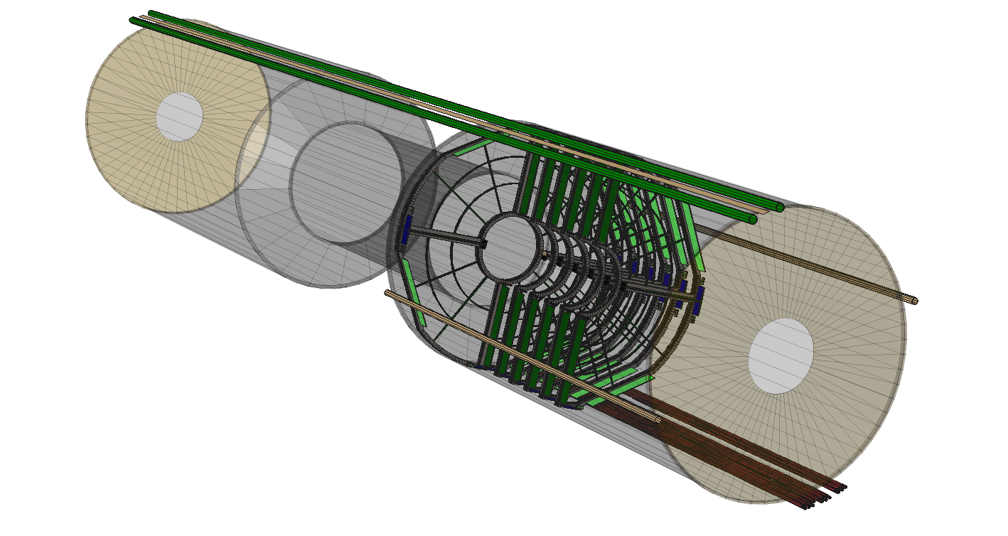

Page maintained by Jason Webb <jwebb@bnl.gov>

AgML Example: The Beam Beam Counters

<Document  file="StarVMC/Geometry/BbcmGeo/BbcmGeo.xml">
<!-- 
  Every AgML document begins with a Document tag, which takes a single "file" 
  attribute as its arguement.
 
  -->
 
 
<Module name="BbcmGeo" comment=" is the Beam Beam Counter Modules GEOmetry "  >
<!-- 
  The Module tag declares an AgML module.  The name should consist of a four
  letter acronym, followed by the word "geo" and possibly a version number.
 
  e.g. BbcmGeo, EcalGeo6, TpceGeo3a, etc...
 
  A mandatory comment attribute provides a short description of which detector
  is implemented by the module.
 
  -->
 
  <Created date="15 march 2002"   />
  <Author  name="Yiqun Wang"      />
  <!-- The Created and Author tags accept a free-form date and author, for the
       purposes of documentation. -->
 
 
  <CDE>AGECOM,GCONST,GCUNIT</CDE>
  <!-- The CDE tag provides some backwards compatability features with starsim.
       AGECOM,GCCONST and GCUNIT are fine for most modules. -->
       
  <Content>BBCM,BBCA,THXM,SHXT,BPOL,CLAD</Content>
  <!-- The Content tag should declare the names of all volumes which are 
       declared in the detector module.  A comma-separated list.  -->
       
  <Structure name="BBCG"  >
    <var name="version"  />
    <var name="onoff(3)" />
    <var name="zdis(2)"  />
  </Structure>
  <!-- The structure tag declares an AgML structure.  It is similar to a c-
       struct, but has some important differences which will be illustrated 
       later.  The members of a Structure are declared using the var tag.  By 
       default, the type of a var will be a float.
 
       Arrays are declared by enclosing the dimensions of the array in 
       parentheses.  Only 1D and 2D arrayes are supported.  e.g.
 
       <var name="x(3)"     />   allowed
       <var name="y(3,3)"   />   allowed
       <var name="z(4,4,4)" />   not allowed
 
       Types may be declared explicitly using the type parameter as below.  
       Valid types are int, float and char.  char variables should be limited 
       to four-character strings for backwards compatability with starsim.  
       Arrays of chars are allowed, in which case you may treat the variable 
       as a string of length Nx4, where N is the dimension of the array.
 
       -->
       
  <Structure name="HEXG">
    <var name="type"    type="float"  />
    <var name="irad"    type="float"  />
    <var name="clad"    type="float"  />
    <var name="thick"   type="float"  />
    <var name="zoffset" type="float"  />
    <var name="xoffset" type="float"  />
    <var name="yoffset" type="float"  />
  </Structure>
       
  <varlist type="float">
     actr,srad,lrad,ztotal,x0,y0,theta0,phi0,xtrip,ytrip,rtrip,thetrip,rsing,thesing
  </varlist>
  <!-- The varlist tag allows you to declare a list of variables of a stated type.
       The variables will be in scope for all volumes declared in the module.
 
       Variables may be initialized using the syntax
            var1/value1/ , var2/value2/, var3, var4/value4/ ...
 
       Arrays of 1 or 2 dimensions may also be declared.  The Assign tag may
       be used to assign values to the arrays:
 
       <Assign var="ARRAY" value="{1,2,3,4}" />
       -->
       
  <varlist type="int">I_trip/0/,J_sing/0/</varlist>
       
  <Fill  name="BBCG"    comment="BBC geometry">
    <var name="Version" value="1.0"              comment=" Geometry version "  />
    <var name="Onoff"   value="{3,3,3}"          comment=" 0 off, 1 west on, 2 east on, 3 both on: for BBC,Small tiles,Large tiles "  />
    <var name="zdis"    value="{374.24,-374.24}" comment=" z-coord from center in STAR (715/2+6*2.54+1=373.8) "  />
  </Fill>
  <!-- The members of a structure are filled inside of a Fill block.  The Fill
       tag specifies the name of the structure being filled, and accepts a
       mandatory comment for documentation purposes.
 
       The var tag is used to fill the members of the structure.  In this 
       context, it accepts three arguements:  The name of the structure member,
       the value which should be filled, and a mandatory comment for 
       documentation purposes.
       
       The names of variables, structures and structure members are case-
       insensitive.
 
       1D Arrays are filled using a comma separated list of values contained in 
       curly brackets...
 
       e.g. value="{1,2,3,4,5}"
 
       2D Arrays are filled using a comma and semi-colon separated list of values
 
       e.g. value="{11,12,13,14,15;        This fills an array dimensioned 
                    21,22,23,24,25;        as A(3,5)
                    31,32,33,34,35;}"
 
       -->
       
 
  <Fill name="HEXG" comment="hexagon tile geometry"  >
    <var name="Type"    value="1"     comment="1 for small hex tile, 2 for large tile "  />
    <var name="irad"    value="4.174" comment="inscribing circle radius =9.64/2*sin(60)=4.174 "  />
    <var name="clad"    value="0.1"   comment="cladding thickness "  />
    <var name="thick"   value="1.0"   comment="thickness of tile "  />
    <var name="zoffset" value="1.5"   comment="z-offset from center of BBCW (1), or BBCE (2) "  />
    <var name="xoffset" value="0.0"   comment="x-offset center from beam for BBCW (1), or BBCE (2) "  />
    <var name="yoffset" value="0.0"   comment="y-offset center from beam for BBCW (1), or BBCE (2) "  />
  </Fill>
       
  <Fill name="HEXG" comment="hexagon tile geometry"  >
    <var name="Type"    value="2"      comment="1 for small hex tile, 2 for large tile "  />
    <var name="irad"    value="16.697" comment="inscribing circle radius (4x that of small one) "  />
    <var name="clad"    value="0.1"    comment="cladding of tile "  />
    <var name="thick"   value="1.0"    comment="thickness of tile "  />
    <var name="zoffset" value="-1.5"   comment="z-offset from center of BBCW (1), or BBCE (2) "  />
    <var name="xoffset" value="0.0"    comment="x-offset center from beam for BBCW (1), or BBCE (2) "  />
    <var name="yoffset" value="0.0"    comment="y-offset center from beam for BBCW (1), or BBCE (2) "  />
  </Fill>
       
  <Use struct="BBCG"/>
  <!-- An important difference between AgML structures and c-structs is that 
       only one instance of an AgML structure is allowed in a geometry module,
       and there is no need for the user to create it... it is automatically
       generated.  The Fill blocks store multiple versions of this structure 
       in an external name space.  In order to access the different versions 
       of a structure, the Use tag is invoked.
       
       Use takes one mandatory attribute: the name of the structure to use.  
       By default, the first set of values declared in the Fill block will 
       be loaded, as above.
 
       The Use tag may also be used to select the version of the structure 
       which is loaded.
 
       Example:
          <Use struct="hexg" select="type" value="2" /> 
 
       The above example loads the second version of the HEXG structure 
       declared above.
       
       NOTE: The behavior of a structure is not well defined before the
             Use operator is applied.
       
       -->
 
 
  <Print level="1" fmt="'BBCMGEO version ', F4.2"  >
    bbcg_version  
  </Print>
  <!-- The Print statement takes a print "level" and a format descriptor "fmt".  The
       format descriptor follows the Fortran formatting convention
 
       (n.b. Print statements have not been implemented in ROOT export
             as they utilize fortran format descriptors)
    -->
     
               
  <!-- small kludge x10000 because ROOT will cast these to (int) before computing properties -->
  <Mixture name="ALKAP" dens="1.432"  >
    <Component name="C5" a="12" z="6"  w="5      *10000"  />
    <Component name="H4" a="1"  z="1"  w="4      *10000"  />
    <Component name="O2" a="16" z="8"  w="2      *10000"  />
    <Component name="Al" a="27" z="13" w="0.2302 *10000"  />
  </Mixture>
  <!-- Mixtures and Materials may be declared within the module... this one is not
       a good example, as there is a workaround being used to avoid some issues 
       with ROOT vs GEANT compatability. -->
 
 
  <Use struct="HEXG" select="type" value="1 "  />
     srad   = hexg_irad*6.0;
     ztotal = hexg_thick+2*abs(hexg_zoffset);
 
  <Use struct="HEXG" select="type" value="2 "  />
     lrad   = hexg_irad*6.0;
     ztotal = ztotal+hexg_thick+2*abs(hexg_zoffset);  <!-- hexg_zoffset is negative for Large (type=2) -->
 
  <!-- AgML has limited support for expressions, in the sense that anyhing which
       is not an XML tag is passed (with minimal parsing) directly to the c++ 
       or mortran compiler.  A few things are notable in the above lines.
 
       (1) Lines may be optionally terminated by a ";", but...
       (2) There is no mechanism to break long lines across multiple lines.
       (3) The members of a structure are accessed using an "_", i.e.
 
           hexg_irad above refers to the IRAD member of the HEXG structure
           loaded by the Use tag.
 
       (4) Several intrinsic functions are available: abs, cos, sin, etc... 
       -->
 
  <Create block="BBCM"  />
  <!-- The Create operator creates the volume specified in the  "block" 
       parameter.  When the Create operator is invoked, execution branches
       to the block of code for the specified volume.   In this case, the
       Volume named BBCM below. -->
 
  <If expr="bbcg_OnOff(1)==1|bbcg_OnOff(1)==3">  
 
    <Placement block="BBCM" in="CAVE" 
               x="0" 
               y="0" 
               z="bbcg_zdis(1)"/>
    <!-- After the volume has been Created, it is positioned within another
         volume in the STAR detector.  The mother volume may be specified
         explicitly with the "in" attribute.
 
         The position of the volume is specified using x, y and z attributes.
 
         An additional attribute, konly, is used to indicate whether or
         not the volume is expected to overlap another volume at the same
         level in the geometry tree.  konly="ONLY" indicates no overlap and
         is the default value.  konly="MANY" indicates overlap is possible.
 
         For more info on ONLY vs MANY, consult the geant 3 manual.         
         -->
 
  </If>
       
  <If expr="bbcg_OnOff(1)==2|bbcg_OnOff(1)==3"  >
    <Placement block="BBCM" in="CAVE" 
               x="0" 
               y="0" 
               z="bbcg_zdis(2)">
      <Rotation alphay="180"  />
    </Placement>            
    <!-- Rotations are specified as additional tags contained withn a
         Placement block of code.  The translation of the volume will
         be performed first, followed by any rotations, evaluated in
         the order given. -->
 
 
  </If>
       
  <Print level="1" fmt="'BBCMGEO finished'"></Print>
       
 
<!--
 
  Volumes are the basic building blocks in AgML.  The represent the un-
  positioned elements of a detector setup.  They are characterized by
  a material, medium, a set of attributes, and a shape.
 
  -->
 
 
 
<!--                      === V o l u m e  B B C M ===                      -->
<Volume name="BBCM" comment="is one BBC East or West module">
 
  <Material  name="Air" />
  <Medium    name="standard"  />
  <Attribute for="BBCM" seen="0" colo="7"  />
  <!-- The material, medium and attributes should be specified first.  If
       ommitted, the volume will inherit the properties of the volume which
       created it. 
 
       NOTE: Be careful when you reorganize a detector module.  If you change
             where a volume is created, you potentially change the properties
         which that volume inherits.
 
   -->
 
  <Shape type="tube" 
     rmin="0" 
     rmax="lrad" 
     dz="ztotal/2" />
  <!-- After specifying the material, medium and/or attributes of a volume,
       the shape is specified.  The Shape is the only property of a volume
       which *must* be declared.  Further, it must be declared *after* the
       material, medium and attributes.
 
       Shapes may be any one of the basic 16 shapes in geant 3.  A future 
       release will add extrusions and composite shares to AgMl.
 
       The actual volume (geant3, geant4, TGeo, etc...) will be created at
       this point.
       -->
         
  <Use struct="HEXG" select="type" value="1 "  />
 
  <If expr="bbcg_OnOff(2)==1|bbcg_OnOff(2)==3"  >
    <Create    block="BBCA"  />
    <Placement block="BBCA" in="BBCM" 
           x="hexg_xoffset" 
           y="hexg_yoffset" 
           z="hexg_zoffset"/>    
  </If>
   
  <Use struct="HEXG" select="type" value="2 "  />
 
  <If expr="bbcg_OnOff(3)==1|bbcg_OnOff(3)==3"  >
 
    <Create block="BBCA"/>
    <Placement block="BBCA" in="BBCM" 
           x="hexg_xoffset" 
           y="hexg_yoffset" 
           z="hexg_zoffset"/>
     
  </If>
   
</Volume>
 
<!--                      === V o l u m e  B B C A ===                      -->
<Volume name="BBCA" comment="is one BBC Annulus module"  >
  <Material name="Air"  />
  <Medium name="standard"  />
  <Attribute for="BBCA" seen="0" colo="3"  />
  <Shape type="tube" dz="hexg_thick/2" rmin="hexg_irad" rmax="hexg_irad*6.0"  />
 
  x0=hexg_irad*tan(pi/6.0)
  y0=hexg_irad*3.0
  rtrip = sqrt(x0*x0+y0*y0)
  theta0 = atan(y0/x0)
 
  <Do var="I_trip" from="0" to="5"  >
   
    phi0 = I_trip*60
    thetrip = theta0+I_trip*pi/3.0
    xtrip = rtrip*cos(thetrip)
    ytrip = rtrip*sin(thetrip)
     
    <Create block="THXM"  />
    <Placement in="BBCA" y="ytrip" x="xtrip" z="0" konly="'MANY'" block="THXM"  >
      <Rotation thetaz="0" thetax="90" phiz="0" phiy="90+phi0" phix="phi0"  />
    </Placement>
     
     
  </Do>
   
   
</Volume>
 
<!--                      === V o l u m e  T H X M ===                      -->
<Volume name="THXM" comment="is on Triple HeXagonal Module"  >
  <Material name="Air"  />
  <Medium name="standard"  />
  <Attribute for="THXM" seen="0" colo="2"  />
  <Shape type="tube" dz="hexg_thick/2" rmin="0" rmax="hexg_irad*2.0/sin(pi/3.0)"  />
 
  <Do var="J_sing" from="0" to="2"  >
   
    rsing=hexg_irad/sin(pi/3.0)
    thesing=J_sing*pi*2.0/3.0
    <Create block="SHXT"  />
    <Placement y="rsing*sin(thesing)" x="rsing*cos(thesing)" z="0" block="SHXT" in="THXM"  >
    </Placement>
   
   
  </Do>
 
</Volume>
 
 
<!--                      === V o l u m e  S H X T ===                      -->
<Volume name="SHXT" comment="is one Single HeXagonal Tile"  >
  <Material name="Air"  />
  <Medium name="standard"  />
  <Attribute for="SHXT" seen="1" colo="6"  />
  <Shape type="PGON" phi1="0" rmn="{0,0}" rmx="{hexg_irad,hexg_irad}" nz="2" npdiv="6" dphi="360" zi="{-hexg_thick/2,hexg_thick/2}"  />
 
  actr = hexg_irad-hexg_clad
 
  <Create block="CLAD"  />
  <Placement y="0" x="0" z="0" block="CLAD" in="SHXT"  >
  </Placement>
 
  <Create block="BPOL"  />
  <Placement y="0" x="0" z="0" block="BPOL" in="SHXT"  >
  </Placement>
 
 
</Volume>
 
 
<!--                      === V o l u m e  C L A D ===                      -->
<Volume name="CLAD" comment="is one CLADding of BPOL active region"  >
  <Material name="ALKAP"  />
  <Attribute for="CLAD" seen="1" colo="3"  />
  <Shape type="PGON" phi1="0" rmn="{actr,actr}" rmx="{hexg_irad,hexg_irad}" nz="2" npdiv="6" dphi="360" zi="{-hexg_thick/2,hexg_thick/2}"  />
 
</Volume>
 
 
<!--                      === V o l u m e  B P O L ===                      -->
<Volume name="BPOL" comment="is one Bbc POLystyren active scintillator layer"  >
 
  <Material name="POLYSTYREN"  />
  <!-- Reference the predefined material polystyrene -->
 
  <Material name="Cpolystyren" isvol="1"  />
  <!-- By specifying isvol="1", polystyrene is copied into a new material
       named Cpolystyrene.  A new material is introduced here in order to
       force the creation of a new medium, which we change with parameters
       below. -->
 
  <Attribute for="BPOL" seen="1" colo="4"  />
  <Shape type="PGON" phi1="0" rmn="{0,0}" rmx="{actr,actr}" nz="2" npdiv="6" dphi="360" zi="{-hexg_thick/2,hexg_thick/2}"  />
 
  <Par name="CUTGAM" value="0.00008"  />
  <Par name="CUTELE" value="0.001"  />
  <Par name="BCUTE"  value="0.0001"  />
  <Par name="CUTNEU" value="0.001"  />
  <Par name="CUTHAD" value="0.001"  />
  <Par name="CUTMUO" value="0.001"  />
  <Par name="BIRK1"  value="1.000"  />
  <Par name="BIRK2"  value="0.013"  />
  <Par name="BIRK3"  value="9.6E-6"  />
  <!--
    Parameters are the Geant3 paramters which may be set via a call to
    GSTPar.
    -->
 
  <Instrument block="BPOL">
    <Hit meas="tof"  nbits="16" opts="C" min="0" max="1.0E-6" />
    <Hit meas="birk" nbits="0"  opts="C" min="0" max="10"     />
  </Instrument>
  <!-- The instrument block indicates what information should be saved
       for this volume, and how the information should be packed. -->
 
</Volume>
 
 
</Module>
</Document>
 
 

AgML Tutorials

Getting started developing geometries for the STAR experiment with AgML.

Setting up your local environment

You need to checkout several directories and complie in this order:

$ cvs co StarVMC/Geometry
$ cvs co StarVMC/StarGeometry
$ cvs co StarVMC/xgeometry
$ cvs co pams/geometry
$ cons +StarVMC/Geometry
$ cons

This will take a while to compile, during which time you can get a cup of coffee, or do your laundry, etc...

If you only want to visualize the STAR detector, you can checkout:

$ cvs co StarVMC/Geometry/macros

Once this is done you can visualize STAR geometries using the viewStarGeometry.C macro in AgML 1, and the loadAgML.C macro in AgML 2.0.

$ root.exe
root [0] .L StarVMC/Geometry/macros/viewStarGeometry.C root [1] nocache=true root [2] viewall=true root [3] viewStarGeometry("y2012") 
root [0] .L StarVMC/Geometry/macros/loadAgML.C
root [1] loadAgML("y2016")
root [2] TGeoVolume *cave = gGeoManager->FindVolumeFast("CAVE");
root [3] cave -> Draw("ogl");              // ogl uses open GL viewer

Tutorial #1 -- Creating and Placing Volumes

Start by firing up your favorite text editor... preferably something which does syntax highlighting and checking on XML documents. Edit the first tutorial geometries located in StarVMC/Geometry/TutrGeo ...

$ emacs StarVMC/Geometry/TutrGeo/TutrGeo1.xml

This module illustrates how to create a new detector module, how to create and place a simple volume, and how to create and place multiple copies of that volume. Next, we need to attach this module to a geometry model in order to visualize it. Geometry models (or "tags") are defined in the StarGeo.xml file.

$ emacs StarVMC/Geometry/StarGeo.xml

There is a simple geometry, which only defines the CAVE. It's the first geometry tag called "black hole". You can add your detector here...

xxx

$ root.exe

root [0] .L StarVMC/Geometry/macros/viewStarGeometry.C root [1] nocache=true root [2] viewStarGeometry("test","TutrGeo1");

The "test" geometry tag is a very simple geometry, implementing only the wide angle hall and the cave. All detectors, beam pipes, magnets, etc... have been removed. The second arguement to viewStarGeometry specifies which geometry module(s) are to be built and added to the test geometry. In this case we add only TutrGeo1. (A comma-separated list of geometry modules could be provided, if more than one geometry module was to be built).

Now you can try modifying TutrGeo1. Feel free to add as many boxes in as many positions as you would like. Once you have done this, recompile in two steps

$ cons +StarVMC/Geometry
$ cons

Tutorial #2 -- A few simple shapes, rotations and reflections

The second tutorial geometry is in StarVMC/Geometry/TutrGeo/TutrGeo2.xml. Again, view it using viewStarGeometry.C

$ root.exe
root [0] .L viewStarGeometry.C
root [1] nocache=true
root [2] viewStarGeometry("test","TutrGeo2")

What does the nocache=true statement do? It instructs viewStarGeometry.C to recreate the geometry, rather than load it from a root file created the last time you ran the geometry. By default, if the macro finds a file name "test.root", it will load the geometry from that file to save time. You don't want this since you know that you've changed the geometry.

The second tutorial illustrates a couple more simple shapes: cones and tubes. It also illustrates how to create reflections. Play around with the code a bit, recompile in the normal manner, then try viewing the geometry again.

Tutorial #3 -- Variables and Structures

AgML provides variables and structures. The third tutorial is in StarVMC/Geometry/TutrGeo/TutrGeo3.xml. Open this up in a text editor and let's look at it. We define three variables: boxDX, boxDY and boxDZ to hold the dimensions of the box we want to create. AgML is case-insensitve, so you can write this as boxdx, BoxDY and BOXDZ if you so choose. In general, choose what looks best and helps you keep track of the code you're writing.

Next check out the volume "ABOX". Note how the shape's dx, dy and dz arguements now reference the variables boxDX, boxDY and boxDZ. This allows us to create multiple versions of the volume ABOX. Let's view the geometry and see.

$ root.exe
root [0] .L StarVMC/Geometry/macros/viewStarGeometry.C
root [1] nocache=true
root [2] viewStarGeometry("test","TutrGeo3")

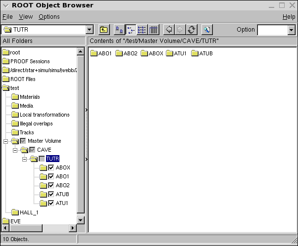
Launch a new TBrowser and open the "test" geometry. Double click test --> Master Volume --> CAVE --> TUTR. You now see all of the concrete volumes which have been created by ROOT. It should look like what you see at the right. We have "ABOX", but we also have ABO1 and ABO2. This demonstrates the an important concept in AgML. Each <Volume ...> block actually defines a volume "factory". It allows you to create multiple versions of a volume, each differing by the shape of the volume. When the shape is changed, a new volume is created with a nickname, where the last letter in the volume name is replaced by [1 2 3 ... 0 a b c ... z] (then the second to last letter, then the third...).

Structures provide an alternate means to define variables. In order to populate the members of a structure with values, you use the Fill statement. Multiple fill statements for a given structure may be defined, providing multiple sets of values. In order to select a given set of values, the <Use ...> operator is invoked. In TutrGeo3, we create and place 5 different tubes, using the data stored in the Fill statements.

However, you might notice in the browser that there are only two concrete instances of the tube being created. What is going on here? This is another feature of AgML. When the shape is changed, AgML will look for another concrete volume with exactly the same shape. If it finds it, it will use that volume. If it doesn't, then a new volume is created.

There's alot going on in this tutorial, so play around a bit with it.

Tutorial #4 -- Some more shapes

AgML vs AgSTAR Comparison

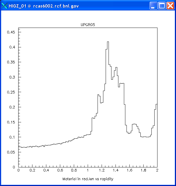
Abstract: We compare the AgML and AgSTAR descriptions of recent revisions of the STAR Y2005 through Y2011 geometry models. We are specifically interested in the suitability of the AgML model for tracking. We therefore plot the material contained in the TPC vs pseudorapidity for (a) all detectors, (b) the time projection chamber, and (c) the sensitive volumes of the time projection chamber. We also plot (d) the material found in front of the TPC active volumes.

Issues with PhmdGeo.xml

Two cases where the AgSTAR parser truncates a line in the phmdgeo.g file. These should be fixed, but need to verify.

Decription of the Plots Below you will find four columns of plots, for the highest revision of each geometry from y2005 to the present. The columns from left-to-right show comparisons of the material budget for STAR and its daughter volumes, the material budgets for the TPC and it's immediate daughter volumes, the material budgets for the active volumes in the TPC, and the material in front of the active volume of the TPC. In the context of tracking, the right-most column is the most important. Each column contains three plots. The top plot shows the material budget in the AgML model. The middle plot, the material budget in the AgSTAR model. The bottom plot shows the difference divided by the AgSTAR model. The y-axis on the difference plot extends between -2.5% and +2.5%. -------------------------------- Attached you will find much more comprehensive set of plots, contained in a TAR file. PDF's for every subsystem in each of the following geometry tags are provided. They show the material budget comparing AgML to AgSTAR for every volume in the subsystem. They also show a difference plot, equal to the difference divided by the average. There is a color-coding scheme. The volume will be coded green if the largest difference is below 1%, red if it exceeds 1% over an extended range. Yellow indicates a missing (mis-named) volume in one or the other geometry, and orange indicates a 1% difference over a small area (likely the result of roundoff error in alignments of the geometries). STAR Y2011 Geometry Tag Issues with TpceGeo3a.xml TPA1 (tpc inner padrow) differences caused by overlap between TPA1 and a thin layer of G10 in the TPC. The padrow overlap is in the "prompt hits" region. We do not (yet) use prompt hits in tracking. Issues with PhmdGeo.xml Two cases where the AgSTAR parser truncates a line in the phmdgeo.g file. These should be fixed, but need to verify.
(a) Material in STAR Detector and daughters	(b) Material in TPC and daughters	(c) Material in TPC active volumes	(d) Material in front of TPC active volumes

STAR Y2010c Geometry Tag Issues with TpceGeo3a.xml TPA1 (tpc inner padrow) differences caused by overlap between TPA1 and a thin layer of G10 in the TPC. The padrow overlap is in the "prompt hits" region. We do not (yet) use prompt hits in tracking. Issues with PhmdGeo.xml Two cases where the AgSTAR parser truncates a line in the phmdgeo.g file. These should be fixed, but need to verify.
(a) Material in STAR Detector and daughters	(b) Material in TPC and daughters	(c) Material in TPC active volumes	(d) Material in front of TPC active volumes

STAR Y2009c Geometry Tag Issues with TpceGeo3a.xml TPA1 (tpc inner padrow) differences caused by overlap between TPA1 and a thin layer of G10 in the TPC. The padrow overlap is in the "prompt hits" region. We do not (yet) use prompt hits in tracking. Issues with PhmdGeo.xml Two cases where the AgSTAR parser truncates a line in the phmdgeo.g file. These should be fixed, but need to verify.
(a) Material in STAR Detector and daughters	(b) Material in TPC and daughters	(c) Material in TPC active volumes	(d) Material in front of TPC active volumes

STAR Y2008e Geometry Tag Global Issues Upstream areas not included in AgML steering routine. Issues with TpceGeo3a.xml TPA1 (tpc inner padrow) differences caused by overlap between TPA1 and a thin layer of G10 in the TPC. The padrow overlap is in the "prompt hits" region. We do not (yet) use prompt hits in tracking. Issues with PhmdGeo.xml Two cases where the AgSTAR parser truncates a line in the phmdgeo.g file. These should be fixed, but need to verify.
(a) Material in STAR Detector and daughters	(b) Material in TPC and daughters	(c) Material in TPC active volumes	(d) Material in front of TPC active volumes

STAR Y2007h Geometry Tag Global Issues Upstream areas not included in AgML steering routine. Issues with TpceGeo3a.xml TPA1 (tpc inner padrow) differences caused by overlap between TPA1 and a thin layer of G10 in the TPC. The padrow overlap is in the "prompt hits" region. We do not (yet) use prompt hits in tracking. Issues with PhmdGeo.xml Two cases where the AgSTAR parser truncates a line in the phmdgeo.g file. These should be fixed, but need to verify. Issues with SVT.
(a) Material in STAR Detector and daughters	(b) Material in TPC and daughters	(c) Material in TPC active volumes	(d) Material in front of TPC active volumes

STAR Y2006g Geometry Tag Global Issues Upstream areas not included in AgML steering routine. Note: TpceGeo2.xml does not suffer from the overlap issue in TpceGeo3a.xml
(a) Material in STAR Detector and daughters	(b) Material in TPC and daughters	(c) Material in TPC active volumes	(d) Material in front of TPC active volumes

STAR Y2005i Geometry Tag Global Issues Upstream areas not included in AgML steering routine. Issues with TpceGeo3a.xml TPA1 (tpc inner padrow) differences caused by overlap between TPA1 and a thin layer of G10 in the TPC. The padrow overlap is in the "prompt hits" region. We do not (yet) use prompt hits in tracking. Issues with PhmdGeo.xml Two cases where the AgSTAR parser truncates a line in the phmdgeo.g file. These should be fixed, but need to verify.
(a) Material in STAR Detector and daughters	(b) Material in TPC and daughters	(c) Material in TPC active volumes	(d) Material in front of TPC active volumes

AgML vs AgSTAR tracking comparison

Attached is a comparison of track reconstruction using the Sti tracker, with AgI and AgML geometries as input.

Interfacing the New Detector with the STAR Big Full Chain

As STAR gradually comes to the end of its AA heavy ion program and more focus are put on polarized pp/pA physics and future ep/eA project at eRHIC era, many upgrades are foreseen to strengthen the detector capability at forward region. These include both the near-term upgrades for polarized pp program, eg. FMS/FSC/FHC calorimeters and FGT/VFGT tracking, and upgrades for eSTAR in about 5 to 10 years. Different detector concepts exist and optimization is needed to fit them in STAR physics and into the current STAR detector system. To reach a proper solution a lot of Monte Carlo (MC) works will be carried out, especially in the STAR simulation framework for its flexibility, robustness and proven performance during the last decade.

During the last 9 months, I have worked with the colleagues at BNL for developing a new detector concept for eSTAR east-side endcap upgrade to identify reliably the recoiled electrons in ep/eA collisions. This detector design consists of several parts and its functionality need be evaluated in the STAR simulation framework. This procedure, including implementing a new detector into the STAR system and then generating/analyzing the MC data, requires quite a few efforts and collaborations with software experts, at least for a “rookie” (like me, who usually analyzes data without many code development). For the purpose to better arrange my own understanding on this and provide a guide for peoples that will do similar jobs in the future, I write this note based on my experience. Many software experts helped me much in dealing all kinds of problems I met in this work. I hope this guide can also relief their burden, to some extent, from being frequently interrupted by new code developer like me (remember they are already over-occupied to maintain the STAR software environment). Since I’m still not a veteran, this simple note will not contain all pieces but only necessary parts, likely most suitable for beginners only.

- Ming Shao (USTC)

Assume you will work on RCF (RACF) because this is the best-maintained place for computing work at STAR. Normally you should work in the evaluation version, since you'll add and tune new detector models which are not part of the current STAR experiment. So please remember type ‘star eval’ before you start. You’d better also create a new directory for this.

> mkdir [your work path]

> cd [your work path]

> star eval

First you should get the STAR detector geometry description, and then add or modify your new detector. STAR has switched to a new Extensible Markup Language (XML), called AgML, to describe its detector system. This is done by

cvs co StarVMC/Geometry

cvs co StarVMC/StarGeometry

cvs co StarVMC/xgeometry

Then you should create a new directory in StarVMC/Geometry, like all other detectors, with its name representing your new detector (usually ‘XXXXGeo’). For example, I added a new detector geometry named ‘EiddGeo’ into this directory, which is intending to identify electrons (Electron ID Detector). In this directory (XXXXGeo), you can create and further modify your new detector geometry in AgML language. You can find an example - StarVMC/Geometry/BBcmGeo/BbcmGeo.xml, which contains very detailed in-line explanation of this language. You can copy and modify it for your new detector, just following the style. More details about AgML can be found at Jason’s webpage (Jason Webb is the AgML expert).

After you finish your modeling of your new detector, try compile it by type ‘cons’ TWICE in your base work directory (the directory containing the StarVMC directory).

> cons

Debug your code if compilation fails until it succeeds all the way to create geometry libraries in the .sl53_gcc432 directory). Then you can check if the geometry of new detector satisfies your expectation by plotting it out. This can be done by modify the macros in the StarVMC/Geometry and execute them in ROOT.

> root.exe (in the base work directory)

> .L StarVMC/Geometry/macros/viewStarGeometry.C

> viewStarGeometry.C(“XXXX”)

XXXX is a geometry tag. An exmaple is shown on the right. The geometry of a new detector - EIDD - is plotted along with the STAR-TPC. Other detectors and magnetic system are omitted.

For related macros modification Jason can provide help. Note: Jason must acknowledge your work so he can modify the geometry tag or create a new one for you.

Once the new detector geometry is fine you may want to run some simulation events, based on GEANT. Before you can really do MC simulation via STARSIM (formerly known as GSTAR), you should make sure you have instrumented sensitive detector and hit digitalization in your detector geometry. Then you can initialize STARSIM by type ‘starsim’ in your work directory. In STARSIM you can execute your kumac macro to generate some MC events. Kumac is PAW based macro, and for a simple test run (eg. with file name ‘testrun.kumac’) it may look like this:

MACRO testrun

DETP geom devE | devE is a tag for eSTAR simulation

GEXE .$STAR_HOST_SYS/lib/xgeometry.so | use local geometry

GCLO all

MODE All SIMU 1 | 0: no secondary; 1: default secondary; 2: save all secondary

GKIN 1 6 2.0 2.0 -1.5 -1.5

gfile o test1.fzd

TRIG 1

RETURN

This macro will generate 1 negative muon from the center of STAR detector with a transverse momentum 2GeV/c, to pseudo-rapidity -1.5. The azimuthal angle is randomly chosen in the range from 0 to 360 degree. The simulated event, with all hits created in the detector system, is then saved into file ‘test1.fzd’. Before you exit STARSIM, you can print out information of this simulation to check your new detector. For example, you can print all hits created in the detector system by

> gprin hits

The STARSIM manual can be found at this URL. A built-in help command in STARSIM can also help in some details. Just type ‘help’ in STARSIM and follow the help instruction. The section 14 (GEANT related commands), 15 (GSTAR user commands) and 16 (advance GEANT user interface) in the help may be especially important to read.

If you find the generated hits reasonable and want to go forward, you need check out and modify necessary codes in the 'pams' directory, where codes transferring GEANT hits from STARSIM to STAR compatible hit type, are contained. You need at your work directory do

> cvs co pams

The codes contained in 'pams/sim' are especially useful for simulation purpose. Several files at different locations are then to be added or changed. You need create your own hit type in pams/sim/idl directory, where all kinds of hit types are defined. The file name is usually g2t_XXX_hit.idl (XXX is a three character name representing your detector). If your hit type is similar to those already exists, you can also just use that hit type (so no new hit type is needed). For example, a new hit type ‘g2t_etr_hit.idl’ was created when I tried to add a new detector (EiddGeo) into STAR.

struct g2t_etr_hit { /* G2t_etr_hit */

long id; /* primary key */

long next_tr_hit_p;/* Id of next hit on same track */

long track_p; /* Id of parent track */

long volume_id; /* STAR volume identification */

float de; /* energy deposition at hit */

float ds; /* path length within padrow */

float p[3]; /* local momentum */

float tof; /* time of flight */

float x[3]; /* coordinate (Cartesian) */

float lgam; /* ALOG10(GEKin/AMass) */

float length; /* track length up to this hit */

float adc; /* signal in ADC after digitization */

float pad; /* hit pad position used in digitization */

float timebucket; /* hit time position -"- */

};

This hit type is basically the same as TPC hit type since their functionality is similar. If you want this hit be associated with a track, you need also modify the g2t_track.idl in the same directory. Just add two line in the g2t_track struct.

long hit_XXX_p; /* Id of first XXX hit on track linked list */

and

long n_XXX_hit; /* Nhits on XXX */

Several other files necessary to be changed are located at another directory pams/sim/g2t. These files are g2t_XXX.idl, g2t_XXX.F and g2t_volume_id.g (XXX is a three character name representing your detector). g2t_XXX.idl connects g2t_track and your hit type (g2t_XXX_hit.idl) to your detector and g2t_XXX.F implements the actual function. One can refer to codes from detectors with similar functionalities to write your code. For example, g2t_tpc.F is a tracking type detector with energy loss of the track, g2t_tof.F is for timing and g2t_emc.F deals with properties of calorimeter type detector. You should basically follow the style in these example files and just make necessary changes (mostly detector names) related to your detector. For g2t_XXX.idl, an example is

#include "PAM.idl"

#include "g2t_track.idl"

#include "g2t_XXX_hit.idl"

interface g2t_XXX : amiModule{ STAFCV_T call (inout g2t_track g2t_track,

out g2t_XXX_hit g2t_XXX_hit ); };

For g2t_XXX.F, there is one important line in this file ‘call G2R_GET_SYS ('XXXX','YYYY',Iprin,Idigi)’, where XXXX is your detector name already shown in your geometry description ‘XXXXGeo.xml’, and YYYY is the sensitive volume name in your geometry. For example, it’s ‘call G2R_GET_SYS ('EIDD','TABD',Iprin,Idigi)’ in g2t_etr.F, since the corresponding sensitive volume is ‘TABD’ in ‘EiddGeo.xml’.

The g2t_volume_id.g file must also be modified to identify the new detector sensitive volumes, in an unambiguous way. You need provide an unique volume_id for each sensitive volume based on the hit volume id in GEANT, contained in an array numbv. In GEANT, a touchable volume can be uniquely found from its volume architecture. This volume architecture is smartly stored in the array numbv. Unnecessary part of the architecture is omitted provided the sensitive volume can still be located unambiguously. Assume a volume architecture of A containing B, B containing C, C containing D1 and D2, both of which are sensitive. Then numbv only store the volume id of D1 and D2, ie. only 1 number, since A, B and C are the same for D1/D2. However, if B contains another sensitive volume D3 (parallel to C), numbv will contain 2 number for a hit so that D1/D2/D3 can be uniquely identified. You should use the numbers in numbv to form a final volume_id value, eg.

elseif (Csys=='etr') then

sector = MOD( (numbv(1)-1), 12 ); "Sectors count from 0 - 11"

layer = (numbv(1)-1)/ 12; "Layers count from 0 - 2"

section = numbv(2) - 1; "Sections count from 0 - 29"

volume_id = section + 100*layer + 10000*sector

Please note numbv array element start from 1, not 0. Refer to other volume_id’s in the g2t_volume_id.g file.

When these modifications are successfully done, you need re-compile once again, by just type

> cons

in your work directory. WARNING: when you compile pams with your new detector items for the first time, you’re likely to get errors like “.sl53_gcc432/obj/pams/sim/g2t/St_g2t_XXX_Module.cxx:2:31: error: St_g2t_XXX_Module.h: No such file or directory” (XXX is your new detector). If you try “cons” again, the errors may disappear and your compilation seems to end good. However, there might be hidden vulnerability in your compiled code, which may sometimes cause execution problem. So here is a trick – when you meet such errors, clean your previous compilation first, then do the following in correct order.

> cons +pams/sim
> cons +pams
> cons +StarVMC/Geometry
> cons

In this way you can get correctly compiled code.

From now on, when you generate your simulation events in STARSIM, the correct type of hits in your new detector will be saved in the GEANT output file. However, the GEANT file is not plainly readable. The code in STAR software framework to read these data is the St_geant_Maker, which is always contained in the StRoot modular. You should check it out from the library,

> cvs co StRoot/St_geant_Maker

The major file you need to modify is St_geant_Maker.cxx. Its header file St_geant_Maker.h can be often left as it is. The following changes are necessary.

Add a line ‘#include "g2t/St_g2t_XXX_Module.h"’ to the header part of the file (XXX represents your detector abbreviation, as defined in pams/sim/g2t). You needn’t worry about this header file since it is automatically generated when you compile pams.

Add a part of code to read the hits from your detector to STAR TDataSet. An example to add ‘etr’ hits is shown as below.

nhits = 0;

geant3 -> Gfnhit("EIDH","TABD", nhits);

if ( nhits > 0 )

{

St_g2t_etr_hit *g2t_etr_hit = new St_g2t_etr_hit("g2t_etr_hit",nhits);

m_DataSet->Add(g2t_etr_hit);

iRes = g2t_etr( g2t_track, g2t_etr_hit);

if ( Debug() > 1 ) g2t_etr_hit->Print(0,10);

}

Just replace ‘etr’ to your hit type. One attention must be paid to the line ‘geant3 -> Gfnhit("EIDH","TABD", nhits)’. Here EIDH and TABD represent the names of the detector and sensitive volume. However, the actual detector name EIDD is changed to EIDH. This is the protocol – replace the last character of the detector name to ‘H’ (this also means the first 3 characters of your detector name should differ from all other detectors to avoid ambiguity).

The data retrieved from the GEANT files should now be written out for further processing. As a first step, the simulation events are usually stored in StMcEvent, a STAR class dedicated for record MC events. You should start by checking out this class to your work directory.

> cvs co StRoot/StMcEvent

> cvs co StRoot/StMcEventMaker

The second calss ‘StMcEventMaker’, as its name suggested, is intended to write out all necessary information from GEANT simulation to StMcEvent.

There are several classes in the directory StRoot/StMcEvent for you to add and modify. The first 2 classes are your detector hit definition class and collector class, usually with names like StMcXXXHit and StMcXXXHitCollection, where XXX represents your detector. You can refer to other classes in StRoot/StMcEvent with similar function to your detector, or even just use an existing one if you feel it already contains all information you need. For myself, I create 4 new classes StMcEtrHit, StMcEtrHitCollection, StMcEtfHit and StMcEtfHitCollection, at the same time use 2 existing class StMcCalorimeterHit and StMcEmcHitCollection, to implement my EIDD detector.

Then you should add your hit collector to StMcEvent class. In StMcEvent.hh file, add a line

class StMcXXXHitCollection;

to the header part of this file. Then add your hit collector to StMcEvent class protected member

StMcXXXHitCollection* mXXXHits;

and corresponding ‘Get’ and ‘Set’ methods to public function member, respectively

StMcXXXHitCollection* XXXHitCollection() { return mXXXHits; }

const StMcXXXHitCollection* XXXHitCollection() const { return mXXXHits; }

void setXXXHitCollection(StMcXXXHitCollection*);

Again here XXX is for your new detector name. Next in StMcEvent.cc file, add include files

#include "StMcXXXHitCollection.hh"

#include "StMcXXXHit.hh"

to the header part. Add a initialization call

mXXXHits = new StMcXXXHitCollection();

in the function ‘void StMcEvent::makeColls()’. Implement the ‘Set’ method declared in the StMcEvent.hh file

void StMcEvent::setXXXHitCollection(StMcXXXHitCollection* val)

{

if (mXXXHits && mXXXHits!= val) delete mXXXHits;

mXXXHits = val;

}

You may also want to print out your hits in some cases to check if they are OK. So in

void StMcEvent::Print(Option_t *option) const

function, you need a line or more to do this job. Usually it looks like

PrintHeader(Name,name);

PrintHitCollection(Name,name);

where PrintHeader and PrintHitCollection are C++ macros defined in StMcEvent.cc file, and Name/name represent your detector name. There are more than one such macros so you can choose the one best suits your case.

The detector hits caused by charged particles are usually related to track class. For simulation events, this is StMcTrack. You may also want to modify this class to have your detector hits in. Similar to StMcEvent class, you need add your hit member in StMcTrack.hh file, as well as ‘Get’, ‘Set’, ‘Add’ and ‘Remove’ methods.

StPtrVecMcXXXHit mXXXHits;

StPtrVecMcXXXHit& XXXHits() { return mXXXHits; }

const StPtrVecMcXXXHit& XXXHits() const { return mXXXHits; }

void setXXXHits(StPtrVecMcXXXHit&);

void addXXXHit(StMcXXXHit*);

void removeXXXHit(StMcXXXHit*);

Then implement them in StMcTrack.cc file. This is quite straightforward - just refer to other detector hit type in this file to see how to do it.

Besids, don’t forget clear the hits in the destructor StMcTrack::~StMcTrack() by adding a line

mXXXHits.clear();

Other methods you may want to implement are:

ostream& operator<<(ostream& os, const StMcTrack& t),

void StMcTrack::Print(Option_t *option) const

const StPtrVecMcHit *StMcTrack::Hits(StDetectorId Id) const

const StPtrVecMcCalorimeterHit *StMcTrack::CalorimeterHits(StDetectorId Id) const

Neither of them is difficult.

You may notice that a vector class type is used in the codes above which is not declared before - StPtrVecMcXXXHit. This is done in another class StMcContainer.hh. You should add several lines in this file in the following order.

class StMcXXXHit;

typedef vector<StMcXXXHit*> StSPtrVecMcXXXHit;

typedef vector<StMcXXXHit*> StPtrVecMcXXXHit;

typedef StPtrVecMcXXXHit::iterator StMcXXXHitIterator;

typedef StPtrVecMcXXXHit::const_iterator StMcXXXHitConstIterator;

Two other classes contains necessary definitions and links you should modify are StMcEventTypes.hh and StMcEventLinkDef.h. In StMcEventTypes.hh add two lines

#include "StMcXXXHit.hh"

#include "StMcXXXHitCollection.hh"

In StMcEventLinkDef.h, the following lines are to be added.

#pragma link C++ function operator<<(ostream&, const StMcXXXHit&);

#pragma link C++ typedef StSPtrVecMcXXXHit;

#pragma link C++ typedef StPtrVecMcXXXHit;

#pragma link C++ typedef StMcXXXHitIterator;

#pragma link C++ typedef StMcXXXHitConstIterator;

#pragma link C++ class vector<StMcXXXHit*>+;

Now the basic structure of adding your new detector hits into StMcEvent class is accomplished. It’s time to modify the StMcEventMaker class for your new detector. In the header file you need add a Boolean member

Bool_t doUseXXX; //!

If you are adding a new detector of calorimeter type, you’re likely to add a method

void fillXXX(St_g2t_emc_hit*); (if you just use emc hit type)

void fillXXX(St_g2t_XXX_hit*); (if you use your own calorimeter hit type)

Then in StMcEventMaker.cxx the following places are to be changed.

Initialize doUseEcl to kTRUE in class constructor.

In StMcEventMaker::Make() function, add

St_g2t_YYY_hit *g2t_XXX_hitTablePointer = (St_g2t_YYY_hit *) geantDstI("g2t_XXX_hit");

One should pay attention to the type St_g2t_YYY_hit. Here YYY is the hit type (g2t_YYY_hit.idl) you used in pams/sim/g2t_XXX.idl. YYY is not necessary the same as XXX, since you can use existing hit type (YYY) for your new detector (XXX).

Then retrieve the hits by

// XXX Hit Tables

g2t_YYY_hit_st *XXXHitTable = 0;

if (g2t_XXX_hitTablePointer)

XXXHitTable = g2t_XXX_hitTablePointer->GetTable();

if (Debug()) cerr << "Table g2t_XXX_hit found in Dataset " << geantDstI.Pwd()->GetName() << endl;

else

if (Debug()) cerr << "Table g2t_XXX_hit Not found in Dataset " << geantDstI.Pwd()->GetName() << endl;

Then fill the hits, either by AddHits(XXX,XXX,XXX) macro, or your own method fillXXX(St_g2t_emc_hit*) or fillXXX(St_g2t_XXX_hit*). Read carefully the methods if you use the existing StMcCalorimeterHit hit type.

Now you can try to compile StRoot by

> cons +StRoot

After all the codes above are successfully compiled, you can proceed to run your GEANT data through BFC chain to generate STAR data, such as .McEvent.root file. The BFC options you choose depends on which detectors you want to include. A simple option example can be

Debug,devE,agml,McEvent,NoSvtIt,NoSsdIt,Idst,Tree,logger,genvtx,tags,IdTruth,geantout,big,fzin,McEvOut

However, if you need full simulation of STAR TPC, you need add many more options such as tpcrs and related database.

Further process on McEvent should be similar to all other MC data based analysis, but with your own detector feature. One example you may refer to is the StMiniMcMaker. You can check it out from STAR class library and make modifications to suit your work. As an example, I plot the hit points generated by TRD (in the EIDD) and TPC with a MC negative muon track at fixed momentum and direction. It's shown on the right.

All work above described are based on simulation. If you want to further implement “real” data type StEvent, you need add or change the classes in StRoot/StEvent. StEvent data should generally base on real experiment, such as a beam test on your new detector prototype. However, there may be needs for it since the functionality of some STAR classes rely on StEvent rather than StMcEvent.

Similar to what you have done for StMcEvent, you need add StXXXHit and StXXXHitCollection classes and attach them to StEvent and other relevant classes. Other auxiliary classes such as StContainers, StEnumerations and StDetectorDefinitions also need your modification too. All these classes are contained in StRoot/StEvent directory.

You also need add your own detector maker under StRoot directory. A recent example is StEtrFastSimMaker, which is a simple maker to add the endcap TRD hits to StEvent for further process. It’s a fast simulation maker since more realistic makers should base on experimental data. Victor add this maker just to test Stv track finding with endcap TRD - a more complicated work for experts only.

List of Default AgML Materials

List of default AgML materials and mixtures. To get a complete list of all materials defined in a geometry, execute AgMaterial::List() in ROOT, once the geometry has been created.

[-]             Hydrogen:  a=     1.01 z=        1 dens=    0.071 radl=      865 absl=      790 isvol= <unset>  nelem=        1
[-]            Deuterium:  a=     2.01 z=        1 dens=    0.162 radl=      757 absl=      342 isvol= <unset>  nelem=        1
[-]               Helium:  a=        4 z=        2 dens=    0.125 radl=      755 absl=      478 isvol= <unset>  nelem=        1
[-]              Lithium:  a=     6.94 z=        3 dens=    0.534 radl=      155 absl=      121 isvol= <unset>  nelem=        1
[-]            Berillium:  a=     9.01 z=        4 dens=    1.848 radl=     35.3 absl=     36.7 isvol= <unset>  nelem=        1
[-]               Carbon:  a=    12.01 z=        6 dens=    2.265 radl=     18.8 absl=     49.9 isvol= <unset>  nelem=        1
[-]             Nitrogen:  a=    14.01 z=        7 dens=    0.808 radl=     44.5 absl=     99.4 isvol= <unset>  nelem=        1
[-]                 Neon:  a=    20.18 z=       10 dens=    1.207 radl=       24 absl=     74.9 isvol= <unset>  nelem=        1
[-]            Aluminium:  a=    26.98 z=       13 dens=      2.7 radl=      8.9 absl=     37.2 isvol= <unset>  nelem=        1
[-]                 Iron:  a=    55.85 z=       26 dens=     7.87 radl=     1.76 absl=     17.1 isvol= <unset>  nelem=        1
[-]               Copper:  a=    63.54 z=       29 dens=     8.96 radl=     1.43 absl=     14.8 isvol= <unset>  nelem=        1
[-]             Tungsten:  a=   183.85 z=       74 dens=     19.3 radl=     0.35 absl=     10.3 isvol= <unset>  nelem=        1
[-]                 Lead:  a=   207.19 z=       82 dens=    11.35 radl=     0.56 absl=     18.5 isvol= <unset>  nelem=        1
[-]              Uranium:  a=   238.03 z=       92 dens=    18.95 radl=     0.32 absl=       12 isvol= <unset>  nelem=        1
[-]                  Air:  a=    14.61 z=      7.3 dens= 0.001205 radl=    30400 absl=    67500 isvol= <unset>  nelem=        1
[-]               Vacuum:  a=    14.61 z=      7.3 dens=    1e-06 radl= 3.04e+07 absl= 6.75e+07 isvol= <unset>  nelem=        1
[-]              Silicon:  a=    28.09 z=       14 dens=     2.33 radl=     9.36 absl=     45.5 isvol= <unset>  nelem=        1
[-]            Argon_gas:  a=    39.95 z=       18 dens=    0.002 radl=    11800 absl=    70700 isvol= <unset>  nelem=        1
[-]         Nitrogen_gas:  a=    14.01 z=        7 dens=    0.001 radl=    32600 absl=    75400 isvol= <unset>  nelem=        1
[-]           Oxygen_gas:  a=       16 z=        8 dens=    0.001 radl=    23900 absl=    67500 isvol= <unset>  nelem=        1
[-]           Polystyren:  a=   11.153 z=    5.615 dens=    1.032 radl= <unset>  absl= <unset>  isvol= <unset>  nelem=        2
                                                                                           A           Z         W
                                                                                    C   12.000      6.000     0.923
                                                                                    H    1.000      1.000     0.077
[-]         Polyethylene:  a=   10.427 z=    5.285 dens=     0.93 radl= <unset>  absl= <unset>  isvol= <unset>  nelem=        2
                                                                                           A           Z         W
                                                                                    C   12.000      6.000     0.857
                                                                                    H    1.000      1.000     0.143
[-]                Mylar:  a=    12.87 z=    6.456 dens=     1.39 radl= <unset>  absl= <unset>  isvol= <unset>  nelem=        3
                                                                                           A           Z         W
                                                                                    C   12.000      6.000     0.625
                                                                                    H    1.000      1.000     0.042
                                                                                    O   16.000      8.000     0.333

Production Geometry Tags

This page was merged with STAR Geometry in simulation & reconstruction and maintained by STAR's librarian.

Attic

Retired Simulation Pages kept here.

Action Items

Immediate action items:

Y2008 tag
- find out about the status of the FTPC (can't locate the relevant e-mail now)
- find out about the status of PMD in 2008 (open/closed)
- ask Akio about possible updates of the FMS code, get the final version
- based on Dave's records, add a small amount of material to the beampipe
- review the tech drawings from Bill and Will and others and start coding the support structure
- extract information from TOF people about the likely configuration
- when ready, produce the material profile plots for Y2008 in slices in Z
TUP tags
- work with Jim Thomas, Gerrit and primarily Spiros on the definition of geometry for the next TUP wave
- coordinate with Spiros, Jim and Yuri a possible repass of the trecent TUP MC data without the IST
Older tags
- check the more recent correction to the SVT code (carbon instead of Be used in the water channels)
- provide code for the correction for 3 layers of mylar on the beampipe as referred to above in Y2008
- check with Dave about the dimensions of the water channels (likely incorrect in GEANT)
- determine which years we will choose to retrofit with improved SVT (ask STAR members)
MTD
- Establish a new UPGRXX tag for the MTD simulation
- supervise and help Lijuan in extending the filed map
- provide facility for reading a separate map in starsim and root4star (with Yuri)
Misc
- collect feedback on possible simulation plans for the fall'07
- revisit the codes for event pre-selection ("hooks")
- revisit the event mixing scripts
Development
- create a schema to store MC run catalog data with a view to automate job definition (Michael has promised help)

Beampipe support geometry and other news

Documentation for the beampipe support geometry description development

After the completion of the 2007 run, the SVT and the SSD were removed from the STAR detector along with there utility lines. The support structure for the beampipe remained, however.

The following drawings describe the structure of the beampipe support as it exists in the late 2007 and probably throughout 2008

http://drupal.star.bnl.gov/STAR/system/files/BEAMPIPE-SUPPORT.pdf

http://drupal.star.bnl.gov/STAR/system/files/WESTSIDE-1.pdf

http://drupal.star.bnl.gov/STAR/system/files/WESTSIDE-2.pdf

http://drupal.star.bnl.gov/STAR/system/files/WESTSIDE-3.pdf

http://drupal.star.bnl.gov/STAR/system/files/WESTSIDE-4.pdf

http://drupal.star.bnl.gov/STAR/system/files/q060da105b.pdf

http://drupal.star.bnl.gov/STAR/system/files/q060da106.pdf

Further corrections to the SVT geometry model

In the course of recent discussion of the beampipe support and shield material, Dave Lynn has found that even though according to the plans, the material of the cooling water channels in the SVT was specified as Be, in reality carbon composite material was used for that purpose. Below, there are materil vs pseudorapidity plots for the "old" and "new" codes

It can be seen that the difference is of the order of 0.4% rad. length on top of the existing (roughly) 6%. This is enough grounds for cutting a new version of the geometry and will shall create a geometry tag Y2007A which will reflect such change.

Datasets

Here we present information about our datasets.

2005

Description	Dataset name	Statistics, thousands	Status	Moved to HPSS	Comment
Herwig 6.507, Y2004Y	rcf1259	225	Finished	Yes	7Gev<Pt<9Gev
Herwig 6.507, Y2004Y	rcf1258	248	Finished	Yes	5Gev<Pt<7Gev
Herwig 6.507, Y2004Y	rcf1257	367	Finished	Yes	4Gev<Pt<5Gev
Herwig 6.507, Y2004Y	rcf1256	424	Finished	Yes	3Gev<Pt<4Gev
Herwig 6.507, Y2004Y	rcf1255	407	Finished	Yes	2Gev<Pt<3Gev
Herwig 6.507, Y2004Y	rcf1254	225	Finished	Yes	35Gev<Pt<100Gev
Herwig 6.507, Y2004Y	rcf1253	263	Finished	Yes	25Gev<Pt<35Gev
Herwig 6.507, Y2004Y	rcf1252	263	Finished	Yes	15Gev<Pt<25Gev
Herwig 6.507, Y2004Y	rcf1251	225	Finished	Yes	11Gev<Pt<15Gev
Herwig 6.507, Y2004Y	rcf1250	300	Finished	Yes	9Gev<Pt<11Gev
Hijing 1.382 AuAu 200 GeV minbias, 0< b < 20fm	rcf1249	24	Finished	Yes	Tracking,new SVT geo, diamond: 60, +-30cm, Y2005D
Herwig 6.507, Y2004Y	rcf1248	15	Finished	Yes	35Gev<Pt<45Gev
Herwig 6.507, Y2004Y	rcf1247	25	Finished	Yes	25Gev<Pt<35Gev
Herwig 6.507, Y2004Y	rcf1246	50	Finished	Yes	15Gev<Pt<25Gev
Herwig 6.507, Y2004Y	rcf1245	100	Finished	Yes	11Gev<Pt<15Gev
Herwig 6.507, Y2004Y	rcf1244	200	Finished	Yes	9Gev<Pt<11Gev
CuCu 62.4 Gev, Y2005C	rcf1243	5	Finished	No	same as 1242+ keep Low Energy Tracks
CuCu 62.4 Gev, Y2005C	rcf1242	5	Finished	No	SVT tracking test, 10 keV e/m process cut (cf. rcf1237)
10 J/Psi, Y2005X, SVT out	rcf1241	30	Finished	No	Study of the SVT material effect
10 J/Psi, Y2005X, SVT in	rcf1240	30	Finished	No	Study of the SVT material effect
100 pi0, Y2005X, SVT out	rcf1239	18	Finished	No	Study of the SVT material effect
100 pi0, Y2005X, SVT in	rcf1238	20	Finished	No	Study of the SVT material effect
CuCu 62.4 Gev, Y2005C	rcf1237	5	Finished	No	SVT tracking test, pilot run
Herwig 6.507, Y2004Y	rcf1236	8	Finished	No	Test run for initial comparison with Pythia, 5Gev<Pt<7Gev
Pythia, Y2004Y	rcf1235	100	Finished	No	MSEL=2, min bias
Pythia, Y2004Y	rcf1234	90	Finished	No	MSEL=0,CKIN(3)=0,MSUB=91,92,93,94,95
Pythia, Y2004Y, sp.2 (CDF tune A)	rcf1233	308	Finished	Yes	4<Pt<5, MSEL=1, GHEISHA
Pythia, Y2004Y, sp.2 (CDF tune A)	rcf1232	400	Finished	Yes	3<Pt<4, MSEL=1, GHEISHA
Pythia, Y2004Y, sp.2 (CDF tune A)	rcf1231	504	Finished	Yes	2<Pt<3, MSEL=1, GHEISHA
Pythia, Y2004Y, sp.2 (CDF tune A)	rcf1230	104	Finished	Yes	35<Pt, MSEL=1, GHEISHA
Pythia, Y2004Y, sp.2 (CDF tune A)	rcf1229	208	Finished	Yes	25<Pt<35, MSEL=1, GHEISHA
Pythia, Y2004Y, sp.2 (CDF tune A)	rcf1228	216	Finished	Yes	15<Pt<25, MSEL=1, GHEISHA
Pythia, Y2004Y, sp.2 (CDF tune A)	rcf1227	216	Finished	Yes	11<Pt<15, MSEL=1, GHEISHA
Pythia, Y2004Y, sp.2 (CDF tune A)	rcf1226	216	Finished	Yes	9<Pt<11, MSEL=1, GHEISHA
Pythia, Y2004Y, sp.2 (CDF tune A)	rcf1225	216	Finished	Yes	7<Pt<9, MSEL=1, GHEISHA
Pythia, Y2004Y, sp.2 (CDF tune A)	rcf1224	216	Finished	Yes	5<Pt<7, MSEL=1, GHEISHA
Pythia special tune2 Y2004Y, GCALOR	rcf1223	100	Finished	Yes	4<Pt<5, GCALOR
Pythia special tune2 Y2004Y, GHEISHA	rcf1222	100	Finished	Yes	4<Pt<5, GHEISHA
Pythia special run 3 Y2004C	rcf1221	100	Finished	Yes	ENER 200.0, MSEL 2, MSTP (51)=7, MSTP (81)=1, MSTP (82)=1, PARP (82)=1.9, PARP (83)=0.5, PARP (84)=0.2, PARP (85)=0.33, PARP (86)=0.66, PARP (89)=1000, PARP (90)=0.16, PARP (91)=1.0, PARP (67)=1.0
Pythia special run 2 Y2004C (CDF tune A)	rcf1220	100	Finished	Yes	ENER 200.0, MSEL 2, MSTP (51)=7, MSTP (81)=1, MSTP (82)=4, PARP (82)=2.0, PARP (83)=0.5, PARP (84)=0.4, PARP (85)=0.9, PARP (86)=0.95, PARP (89)=1800, PARP (90)=0.25, PARP (91)=1.0, PARP (67)=4.0
Pythia special run 1 Y2004C	rcf1219	100	Finished	Yes	ENER 200.0, MSEL 2, MSTP (51)=7, MSTP (81)=1, MSTP (82)=1, PARP (82)=1.9, PARP (83)=0.5, PARP (84)=0.2, PARP (85)=0.33, PARP (86)=0.66, PARP (89)=1000, PARP (90)=0.16, PARP (91)=1.5, PARP (67)=1.0
Hijing 1.382 AuAu 200 GeV central 0< b < 3fm	rcf1218	50	Finished	Yes	Statistics enhancement of rcf1209 with a smaller diamond: 60, +-30cm, Y2004a
Hijing 1.382 CuCu 200 GeV minbias 0< b < 14 fm	rcf1216	52	Finished	Yes	Geometry: Y2005x
Hijing 1.382 AuAu 200 GeV minbias 0< b < 20 fm	rcf1215	100	Finished	Yes	Geometry: Y2004a, Special D decays

2006

Description	Dataset name	Statistics, thousands	Status	Moved to HPSS	Comment
AuAu 200 GeV central	rcf1289	1	Finished	No	upgr06: Hijing, D0 and superposition
AuAu 200 GeV central	rcf1288	0.8	Finished	No	upgr11: Hijing, D0 and superposition
AuAu 200 GeV min bias	rcf1287	5	Finished	No	upgr11: Hijing, D0 and superposition
AuAu 200 GeV central	rcf1286	1	Finished	No	upgr10: Hijing, D0 and superposition
AuAu 200 GeV min bias	rcf1285	6	Finished	No	upgr10: Hijing, D0 and superposition
AuAu 200 GeV central	rcf1284	1	Finished	No	upgr09: Hijing, D0 and superposition
AuAu 200 Gev min bias	rcf1283	6	Finished	No	upgr09: Hijing, D0 and superposition
AuAu 200 GeV min bias	rcf1282	38	Finished	No	upgr06: Hijing, D0 and superposition
AuAu 200 GeV min bias	rcf1281	38	Finished	Yes	upgr08: Hijing, D0 and superposition
AuAu 200 GeV min bias	rcf1280	38	Finished	Yes	upgr01: Hijing, D0 and superposition
AuAu 200 GeV min bias	rcf1279	38	Finished	Yes	upgr07: Hijing, D0 and superposition
Extension of 1276: D0 superposition	rcf1278	5	Finished	No	upgr07: Z cut=+-300cm
AuAu 200 GeV min bias	rcf1277	5	Finished	No	upgr05: Z cut=+-300cm
AuAu 200 GeV min bias	rcf1276	35	Finished	No	upgr05: Hijing, D0 and superposition
Pythia 200 GeV + HF	rcf1275	23*4	Finished	No	J/Psi and Upsilon(1S,2S,3S) mix for embedding
AuAu 200 GeV min bias	rcf1274	10	Finished	No	upgr02 geo tag, \|eta\|<1.5 (tracking upgrade request)
Pythia 200 GeV	rcf1273	600	Finished	Yes	Pt <2 (Completing the rcf1224-1233 series)
CuCu 200 GeV min bias+D0 mix	rcf1272	50+2508	Finished	Yes	Combinatorial boost of rcf1261, sigma: 60, +-30
Pythia 200 GeV	rcf1233	300	Finished	Yes	4< Pt <5 (rcf1233 extension)
Pythia 200 GeV	pds1232	200	Finished	Yes	3< Pt <4 (rcf1232 clone)
Pythia 200 GeV	pds1231	240	Finished	Yes	2< Pt <3 (rcf1231 clone)
Pythia 200 GeV	rcf1229	200	Finished	Yes	25< Pt <35 (rcf1229 extension)
Pythia 200 GeV	rcf1228	200	Finished	Yes	15< Pt <25 (rcf1228 extension)
Pythia 200 GeV	rcf1227	208	Finished	Yes	11< Pt <15 (rcf1227 extension)
Pythia 200 GeV	rcf1226	200	Finished	Yes	9< Pt <11 (rcf1226 extension)
Pythia 200 GeV	rcf1225	200	Finished	Yes	7< Pt <9 (rcf1225 extension)
Pythia 200 GeV	rcf1224	212	Finished	Yes	5< Pt <7 (rcf1224 extension)
Pythia 200 GeV Y2004Y CDF_A	rcf1271	120	Finished	Yes	55< Pt <65
Pythia 200 GeV Y2004A CDF_A	rcf1270	120	Finished	Yes	45< Pt <55
CuCu 200 GeV min bias	rcf1266	10	Finished	Yes	SVT study: clams and two ladders
CuCu 200 GeV min bias	rcf1265	10	Finished	Yes	SVT study: clams displaced
CuCu 200 GeV min bias	rcf1264	10	Finished	Yes	SVT study: rotation of the barrel
CuCu 62.4 GeV min bias+D0 mix	rcf1262	50*3	Finished	Yes	3 subsets: Hijing, single D0, and the mix
CuCu 200 GeV min bias+D0 mix	rcf1261	50*3	Finished	No	3 subsets: Hijing, single D0, and the mix
1 J/Psi over 200GeV minbias AuAu	rcf1260	10	Finished	No	J/Psi mixed with 200GeV AuAu Hijing Y2004Y 60/35 vertex

2007

Unless stated otherwise, all pp collisions are modeled with Pythia, and all AA collisions with Hijing. Statistics is listed in thousands of events. Multiplication factor in some of the records refelcts the fact that event mixing was done for a few types of particles, on the same base of original event files.

Name	System/Energy	Statistics	Status	HPSS	Comment	Site
rcf1290	AuAu200 0<b<3fm, Zcut=5cm	32*5	Done	Yes	Hijing+D0+Lac2+D0_mix+Lac2_mix	rcas
rcf1291	pp200/UPGR07/Zcut=10cm	10	Done	Yes	ISUB = 11, 12, 13, 28, 53, 68	rcas
rcf1292	pp500/UPGR07/Zcut=10cm	10	Done	Yes	ISUB = 11, 12, 13, 28, 53, 68	rcas
rcf1293	pp200/UPGR07/Zcut=30cm	205	Done	Yes	ISUB = 11, 12, 13, 28, 53, 68	rcas
rcf1294	pp500/UPGR07/Zcut=30cm	10	Done	Yes	ISUB = 11, 12, 13, 28, 53, 68	rcas
rcf1295	AuAu200 0<b<20fm, Zcut=30cm	20	Done	Yes	QA run for the Y2007 tag	rcas
rcf1296	AuAu200 0<b<3fm, Zcut=10cm	100*5	Done	Yes	Hijing,B0,B+,B0_mix,B+_mix, Y2007	rcas
rcf1297	AuAu200 0<b<20fm, Zcut=300cm	40	Done	Yes	Pile-up simulation in the TUP studies, UPGR13	rcas
rcf1298	AuAu200 0<b<3fm, Zcut=15cm	100*5	Done	Part	Hijing,D0,Lac2,D0_mix,Lac2_mix, UPGR13	rcas
rcf1299	pp200/Y2005/Zcut=50cm	800	Done	Yes	Pythia, photon mix, pi0 mix	rcas
rcf1300	pp200/UPGR13/Zcut=15cm	100	Done	No	Pythia, MSEL=4 (charm)	rcas
rcf1301	pp200/UPGR13/Zcut=300cm	84	Done	No	Pythia, MSEL=1, wide vertex	rcas
rcf1302	pp200 Y2006C	120	Done	No	Pythia for Spin PWG, Pt(45,55)GeV	rcas
rcf1303	pp200 Y2006C	120	Done	No	Pythia for Spin PWG, Pt(35,45)GeV	rcas
rcf1304	pp200 Y2006C	120	Done	No	Pythia for Spin PWG, Pt(55,65)GeV	rcas
rcf1296	Upsilon S1,S2,S3 + Hijing	15*3	Done	No	Muon Telescope Detector, ext.of 1296	rcas
rcf1306	pp200 Y2006C	400	Done	Yes	Pythia for Spin PWG, Pt(25,35)GeV	rcas
rcf1307	pp200 Y2006C	400	Done	Yes	Pythia for Spin PWG, Pt(15,25)GeV	rcas
rcf1308	pp200 Y2006C	420	Done	Yes	Pythia for Spin PWG, Pt(11,15)GeV	rcas
rcf1309	pp200 Y2006C	420	Done	Yes	Pythia for Spin PWG, Pt(9,11)GeV	rcas
rcf1310	pp200 Y2006C	420	Done	Yes	Pythia for Spin PWG, Pt(7,9)GeV	rcas
rcf1311	pp200 Y2006C	400	Done	Yes	Pythia for Spin PWG, Pt(5,7)GeV	rcas
rcf1312	pp200 Y2004Y	544	Done	No	Di-jet CKIN(3,4,7,8,27,28)=7,9,0.0,1.0,-0.4,0.4	rcas
rcf1313	pp200 Y2004Y	760	Done	No	Di-jet CKIN(3,4,7,8,27,28)=9,11,-0.4,1.4,-0.5,0.6	rcas
rcf1314	pp200 Y2004Y	112	Done	No	Di-jet CKIN(3,4,7,8,27,28)=11,15,-0.2,1.2,-0.6,-0.3	Grid
rcf1315	pp200 Y2004Y	396	Done	No	Di-jet CKIN(3,4,7,8,27,28)=11,15,-0.5,1.5,-0.3,0.4	Grid
rcf1316	pp200 Y2004Y	132	Done	No	Di-jet CKIN(3,4,7,8,27,28)=11,15,0.0,1.0,0.4,0.7	Grid
rcf1317	pp200 Y2006C	600	Done	Yes	Pythia for Spin PWG, Pt(4,5)GeV	Grid
rcf1318	pp200 Y2006C	690	Done	Yes	Pythia for Spin PWG, Pt(3,4)GeV	Grid
rcf1319	pp200 Y2006C	690	Done	Yes	Pythia for Spin PWG, Minbias	Grid
rcf1320	pp62.4 Y2006C	400	Done	No	Pythia for Spin PWG, Pt(4,5)GeV	Grid
rcf1321	pp62.4 Y2006C	250	Done	No	Pythia for Spin PWG, Pt(3,4)GeV	Grid
rcf1322	pp62.4 Y2006C	220	Done	No	Pythia for Spin PWG, Pt(5,7)GeV	Grid
rcf1323	pp62.4 Y2006C	220	Done	No	Pythia for Spin PWG, Pt(7,9)GeV	Grid
rcf1324	pp62.4 Y2006C	220	Done	No	Pythia for Spin PWG, Pt(9,11)GeV	Grid
rcf1325	pp62.4 Y2006C	220	Done	No	Pythia for Spin PWG, Pt(11,15)GeV	Grid
rcf1326	pp62.4 Y2006C	200	Running	No	Pythia for Spin PWG, Pt(15,25)GeV	Grid
rcf1327	pp62.4 Y2006C	200	Running	No	Pythia for Spin PWG, Pt(25,35)GeV	Grid
rcf1328	pp62.4 Y2006C	50	Running	No	Pythia for Spin PWG, Pt(35,45)GeV	Grid

2009

qqqqqqqqqqqqqqqqqqqqqqqqqqq

Name	SystemEnergy	Range	Statistics	Comment
rcf9001	pp200, y2007g	03_04gev	690k	Jet Study AuAu200(PP200) JLC PWG
rcf9002		04_05gev	686k
rcf9003		05_07gev	398k
rcf9004		07_09gev	420k
rcf9005		09_11gev	412k
rcf9006		11_15gev	420k
rcf9007		15_25gev	397k
rcf9008		25_35gev	400k
rcf9009		35_45gev	120k
rcf9010		45_55gev	118k
rcf9011		55_65gev	120k

Name	SystemEnergy	Range	Statistics	Comment
rcf9021	pp200,y2008	03_04 GeV	690k	Jet Study AuD200(PP200) JLC PWG
rcf9022		04_05 GeV	686k
rcf9023		05_07 GeV	398k
rcf9024		07_09 GeV	420k
rcf9025		09_11 GeV	412k
rcf9026		11_15 GeV	420k
rcf9027		15_25 GeV	397k
rcf9028		25_35 GeV	400k
rcf9029		35_45 GeV	120k
rcf9030		45_55 GeV	118k
rcf9031		55_99 GeV	120k

Name	SystemEnergy	Range	Statistics	Comment
rcf9041	PP500, Y2009	03_04gev	500k	Spin Study PP500 Spin group(Matt,Jim,Jan) 2.3M evts
rcf9042		04_05gev	500k
rcf9043		05_07gev	300k
rcf9044		07_09gev	250k
rcf9045		09_11gev	200k
rcf9046		11_15gev	100k
rcf9047		15_25gev	100k
rcf9048		25_35gev	100k
rcf9049		35_45gev	100k
rcf9050		45_55gev	25k
rcf9051		55_99gev	25k

rcf9061	CuCu200,y2005h	B0_14	200k	CuCu200 radiation length budget, Y.Fisyak, KyungEon Choi.
rcf9062	AuAu200, y2007h	B0_14	150k	AuAu200 radiation length budget Y.Fisyak ,KyungEon Choi

2010

Information on Monte Carlo Data Samples

You do not have access to view this node

Geometry	y2009a
Library	SL09g
Generator	Pythia 6.4.22
Tune	320
Field	-5.0
ETA	-10 < η < +10
PHI	-π < φ < +π
vertex	0, 0, -2
width	0.015, 0.015, 42.0

Sample	Channel	Events
rcf10000	W⁺ → e+ nu	10k
rcf10001	W^- → e- nu	6k
rcf10002	W⁺ → tau+ nu W^- → tau- nu	10k
rcf10003	pp → W^+/- + jet	10k
rcf10004	Z e+e-, no Z/gamma interference	4k
rcf10005	Z all but e+e-	10k
rcf10006	QCD w/ partonic pT > 35 GeV	100k

Geometry Tag Options

This page documents the options in geometry.g which define each of the production tags.

Geometry Tag Options II

The attached spreadsheets document the production tags in STARSIM on 11/30/2009. At that time the y2006h and y2010 tags were in development and not ready for production.

Material Balance Histograms

Y2008a

y2008a full and TPC only material histograms

y2008aStar

1	2

y2008aTpce

y2005g

y2005gStar

	2
3

y2005gTpce

y2008yf

y2008yfStar

	111

	`

y2008yfTpce

	1

y2009

y2009Star

	.
	.

y2009Tpce

	.

STAR AgML Geometry Comparison with STARSIM/AgSTAR

STAR Geometry Comparison: AgML vs AgSTAR

At the left is a general status for each geometry tag which compiles in AgML. All volumes are tested recursively except for the "IBEM" and similar support structures for the VPD, and the Endcap SMD strips. (The ESMD planes are tested as a unit, rather than test all 2*12*288 SMD strips).

Color codes:

Green: No differences larger than 1%

Yellow: The volume did not appear in AgSTAR geometry

Orange: Difference was larger than 1%, but absolute difference is absolutely negligible.

Red: A difference larger than 1% was detected for a significant amount of material; or a negligible but widespread difference was detected.

At the right is a PDF file for each geometry tag. For each volume we show two plots. The top plot shows the absolute number of radiation lengths which a geantino encounters traversing the geometry, starting at the geometry and following a straight line at the given pseudorapidity. We average over all phi. The left (right) hashes show the AgML (AgSTAR) geometry. The difference (expressed as a fractional value) of the two histograms is shown the lower plot. Frequently the differences are small, e.g. 10^-6, and ROOT rescales the plots accordingly. Since it is difficult to read the scales of so many plots at once, we have color coded the plots. (Coding seems to fail in the generation of some histograms)... The meaning of the color coding is summarized below.

<?php
/********************************************************************** START OF PHP */

/* =======================================================
   Helper function to show the status_yXXXX.png
   ======================================================= */
function showImage( $tag, $dir ) {

   echo "<img src=\"$dir/status_$tag.png\" />";

}

/* =======================================================
   Helper function to show the PDF file
   ======================================================= */
function showGoogle( $tag, $dir ) {
   /*
   echo "<iframe border=\"0\" url=\"http://docs.google.com/gview?url=$dir$tag.pdf&amp;embedded=true\" style=\"width: 562px; height: 705px;\"> </iframe>";
   */

echo

"<iframe frameborder=\"0\" style=\"width: 562px; height: 705px;\" src=\"http://docs.google.com/gview?url=$dir/$tag.pdf&amp;embedded=true\"></iframe>"

;
}


/* =======================================================
   First some PHP input... find the date of the comparison 
   ======================================================= */
$YEAR="2011";
$DATE="06-15-2011";
$DIR="http://www.star.bnl.gov/~jwebb/".$YEAR."/".$DATE."/AgML-Comparison/";
$TAGS=$DIR."TAGS";
/* =======================================================
   Output header for this page 
   ======================================================= */

echo "<h3>STAR AgML vs AgSTAR Comparison on ".$DATE."</h3>";

/* =======================================================
   Read in each line in the TAGs file 
   ======================================================= */
$handle = @fopen("$TAGS", "r");
if ($handle) {
    while (($buffer = fgets($handle, 4096)) !== false) {

        /* Trim the whitespace out of the string */
        $buffer=trim($buffer);

        /* Draw an HRULE and specify which geometry tag we are using */
        echo "<hr><p>STAR Geometry Tag $buffer</p>";

        /* Now build a 2-entry table with the status PNG on the left 
           and the summary PDF ala google docs on the right */

        showImage( $buffer, $DIR );

        showGoogle( $buffer, $DIR );

    }
    if (!feof($handle)) {
        echo "Error: unexpected fgets() fail\n";
    }
    fclose($handle);
}

/************************************************************************ END OF PHP */
?>

STAR AgML Language Reference

STAR Geometry Page

R&D Tags

The R&D conducted for the inner tracking upgrade required that a few specialized geometry tags be created. For a complete set of geometry tags, please visit the STAR Geometry in simulation & reconstruction page. The below serves as additional documentation and details.

Taxonomy:

SSD: Silicon strip detector
IST: Inner Silicon Tracker
HFT: Heavy Flavor Tracker
IGT: Inner GEM Tracker
HPD: Hybrid Pixel Detector

The TPC is present in all configuration listed below and the SVT is in none.

Tag	SSD	IST	HFT	IGT	HPD	Contact Person	Comment
UPGR01	+		+
UPGR02		+	+
UPGR03		+	+	+
~~UPGR04~~	+				+	Sevil	retired
~~UPGR05~~	+	+	+	+	+	Everybody	retired
~~UPGR06~~	+		+		+	Sevil	retired
UPGR07	+	+	+	+		Maxim
~~UPGR08~~		+	+	+	+	Maxim
~~UPGR09~~		+	+		+	Gerrit	retired Outer IST layer only
UPGR10	+	+	+			Gerrit	Inner IST@9.5cm
UPGR11	+	+	+			Gerrit	IST @9.5&@17.0
~~UPGR12~~	+	+	+	+	+	Ross Corliss	retired UPGR05*diff.igt.radii
UPGR13	+	+	+	+		Gerrit	UPGR07(new 6 disk FGT)corrected SSD*(no West Cone)
UPGR14	+		+	+		Gerrit	UPGR13 - IST
UPGR15	+	+	+			Gerrit	Simple Geometry for testing, Single IST@14cm, hermetic/polygon Pixel/IST geometry. Only inner beam pipe 0.5mm Be. Pixel 300um Si, IST 1236umSi
UPGR20	+					Lijuan	Y2007 + one TOF
UPGR21	+					Lijuan	UPGR20 + full TOF

Eta coverage of the SSD and HFT at different vertex spreads:

Z cut, cm	eta SSD	eta HFT
5	1.63	2.00
10	1.72	2.10
20	1.87	2.30
30	2.00	2.55

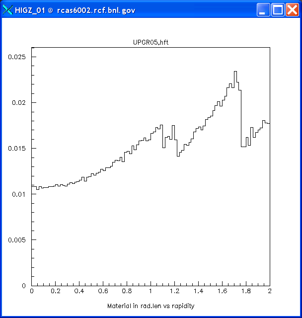
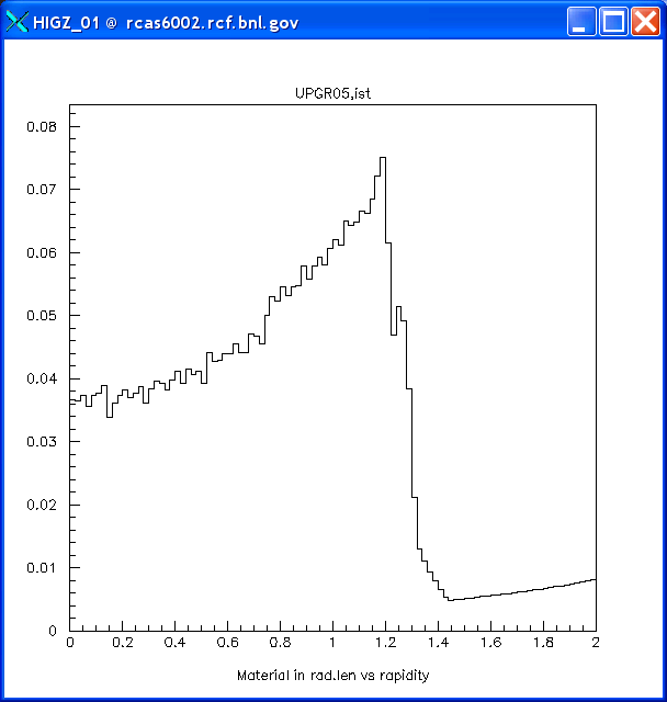
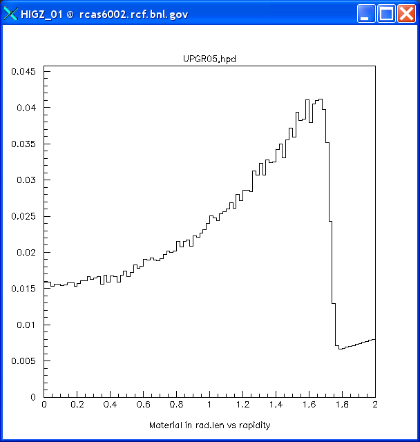
Material balance studies for the upgrade: presented below are the usual radiation length plots (as a function of rapidity).

Full UPGR05:

Forward region: the FST and the IGT ONLY:

Below, we plot the material for each individual detector, excluding the forward region to reduce ambiguity.

SSD:

IST:

HPD:

HFT: