Previously, I summarized our investigation of how to assess the systematic due to secondary vertices in our analysis:

https://drupal.star.bnl.gov/STAR/blog/dmawxc/update-12192019-understanding-turning-decays-vs-run-9-dijet-embedding-sample

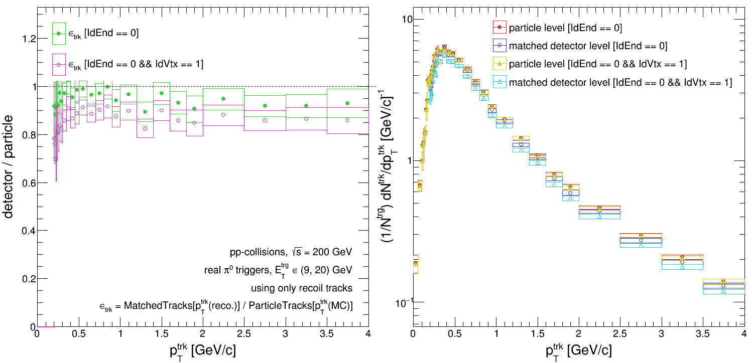
It's worth noting that when we calculate the parameterized detector response (tracking efficiency and tracking resolution) that we apply to our Pythia8 sample, it's calculated with decays on; i.e. that we match reconstructed tracks (satisfying all of our QA cuts) to generated particles which are charged and have [IdEnd == 0] (as defined in the last post).  So what would happen if we calculated the tracking efficiency -- by far what we would expect to be the dominant uncertainty -- for two other cases: [IdVtx == 1] (also defined in the last post), and [IdVtx == 1 && IdEnd == 0]?

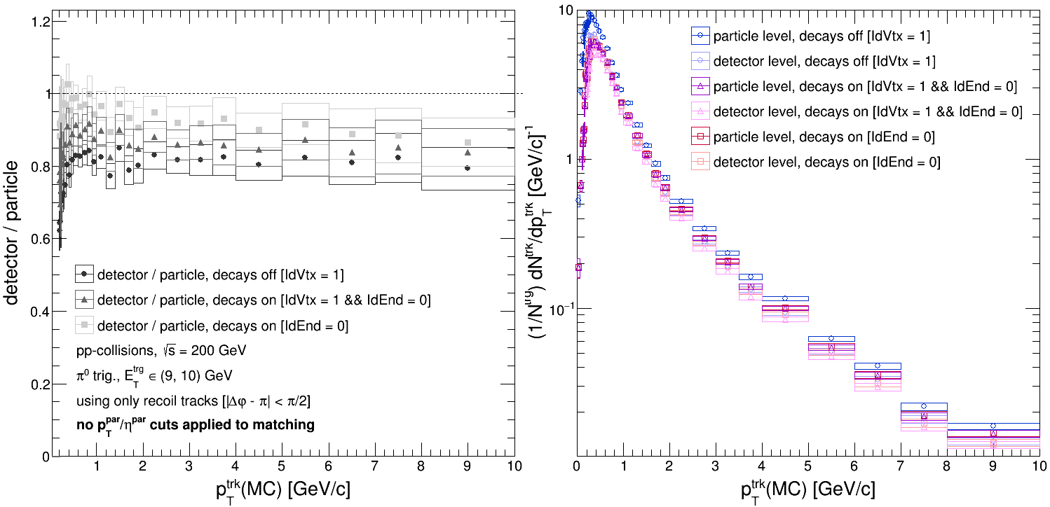
There are substantial differences between all three cases.  We should anticipate that the tracking efficiency for [IdVtx == 1] falls below that for [IdEnd == 0] and [IdEnd == 0 && IdVtx == 1].  In the former case, the set of generated particles we are trying to reconstruct will included resonances and other particles which will decay on length scales smaller than or comparable to our detector.  Thus, it's likely that we'll reconstruct these particles' decay products rather than the particles themselves and so see a lower tracking efficiency.

But what about the other two?  For [IdVtx == 1 && IdEnd == 0], the tracking efficiency peaks at ~90% which is what we might anticipate from previous studies of the Run 9 tracking efficiency.  Yet [IdEnd == 0] gives an efficiency which peaks around ~95%...  This is strange; why should there be such a big difference between these two populations of particles?  After all, the [IdVtx == 1 && IdEnd == 0] is a subset of the [IdEnd == 0] population.  Below shows the tracking efficiency for [IdVtx > 1 && IdEnd == 0] ('IdVtx' should always be greater than or equal to 1).

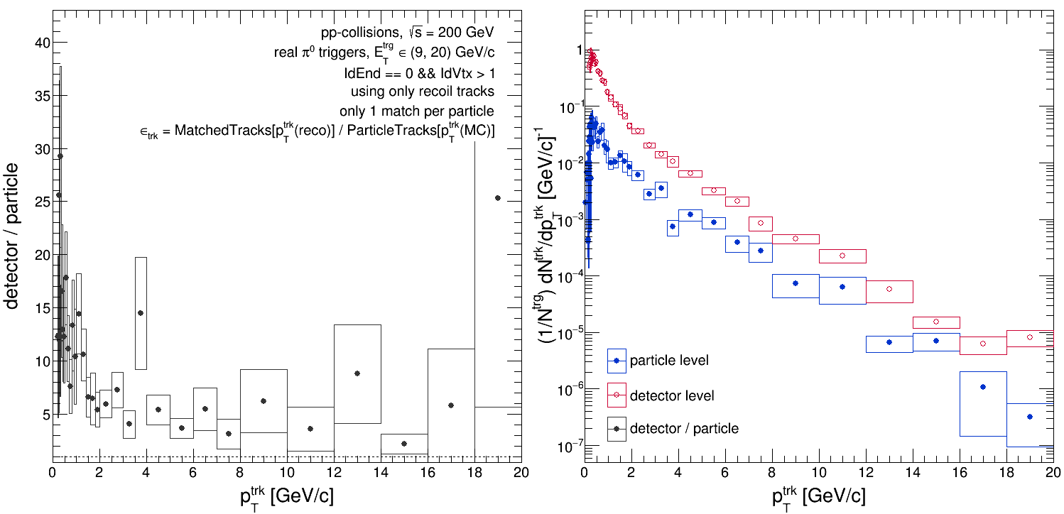
Which is nonsense!  As the text in the plot indicates, this is after restricting each particle to have at most 1 match (there are rare instances where you might find multiple).  So how could it be that the matched tracks have a bigger yield than the particles?  It's worth noting here that the way we're calculating the tracking efficiency is like so:

effTrack = PtMatch{pTreco} / PtParticle{pTmc}

Here 'PtMatch{*}' indicates the matched track spectrum as a function of either 'pTreco' (smeared, detector-level 'pT') or 'pTmc' (unsmeared, particle-level 'pT'), and 'PtParticle{pTmc}' indicates the particle-level track spectrum as a function of 'pTmc'.  In the code, I fill two histograms for 'PtMatch': 'hPtForEff[1]', which is for the 'PtMatch{pTmc}' case, and 'hPtQA[2]', which is for the 'PtMatch{pTreco}' case.  They are filled under the same condition (I've attached screenshots of the code), so what happens if we use 'pTmc' for the numerator rather than 'pTreco'?

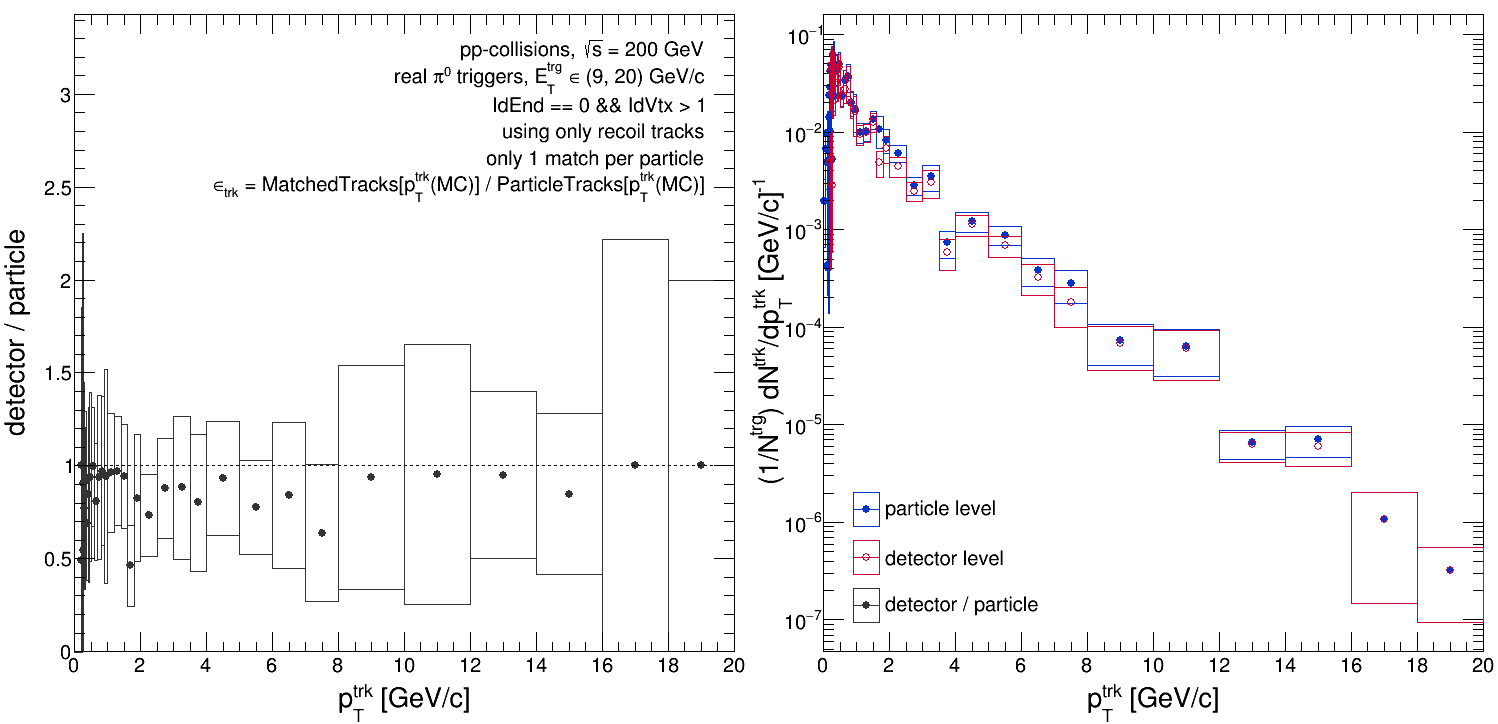
Which looks totally fine!  So it doesn't appear to be a bug in the code...  Just to be clear, this for the case where the tracking efficiency is calculated as so:

effTrack = PtMatch{pTmc} / PtParticle{pTmc}

The following plot shows the two cases, [IdVtx == 1 && IdEnd == 0] vs. [IdEnd == 0], when the tracking efficiency is calculated using 'pTmc' for the numerator.

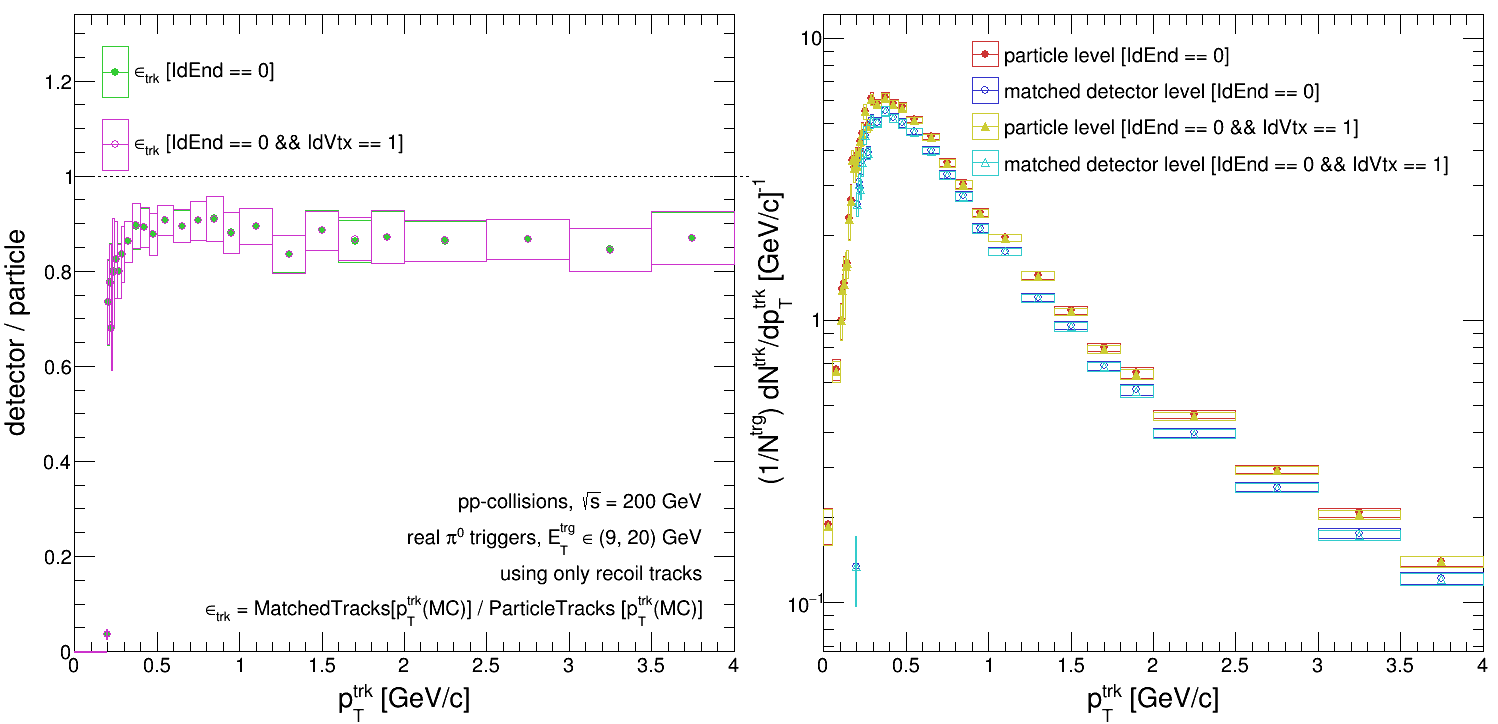
And they agree beautifully!  Again, here's a plot comparing [IdVtx == 1 && IdEnd == 0] to [IdEnd == 0] when we use 'pTreco' for the numerator:

Barring any subtle bugs in the code, this would suggest to me that we have particles originating secondary vertices (decay products and the like) whose reconstructed 'pT' is artificially inflated due to vertexing...  So how do we go about dealing with that?  Is this the best way to assess the systematic due to secondary vertices?

Note: in the code screenshots, I use the variable 'pTmat' to indicate 'pTreco'.  And 'pTmc' is used to indicate 'pTmc'.